for independent, not necessarily identically distributed, positive \(X_i\) and large \(u\). Their method is k-moment tilting (KMT), an importance sampling scheme that tilts each marginal by a power rather than by an exponential:
The reason for a power rather than an exponential is immediate: exponential tilting needs a finite moment generating function, which heavy-tailed laws do not have. A power tilt only needs a finite \(k\)-th moment, so it survives on the Pareto. Since \(g_i/f_i\) is non-decreasing, the tilted variable stochastically dominates the original, which is what fixes the low hit rate.
The paper’s three claims are that KMT (i) applies to heavy- and light-tailed marginals under the general independent non-identically distributed setting, where hazard rate twisting cannot go because it assumes a single common hazard function, (ii) admits closed-form optimal tilting parameters obtained by minimizing a deterministic upper bound rather than the intractable second moment, with a clean characterization of the rare-event threshold \(u_0\) below which no tilting is needed, and (iii) is asymptotically optimal for the Pareto family, and beats the HRT-SOC scheme of Ben Amar et al. (2023) on computational time by roughly 9.6-fold at \(u = 800\).
That last comparison is the thread back to the rest of this group. Ben Amar et al. (2023) is the state-dependent stochastic control method reproduced on its own page, and its weakness, that a backward recursion must be re-solved for each problem, is precisely what KMT is designed to avoid:
KMT determines the optimal tilting parameter \(k^*\) via a one-step procedure, namely by solving a single scalar equation, after which sampling proceeds without further adjustment. Conversely, HRT-SOC’s state-dependent mechanism requires backward recursion and repeated pathwise recomputations, introducing substantial computational overhead that limits its practical efficiency.
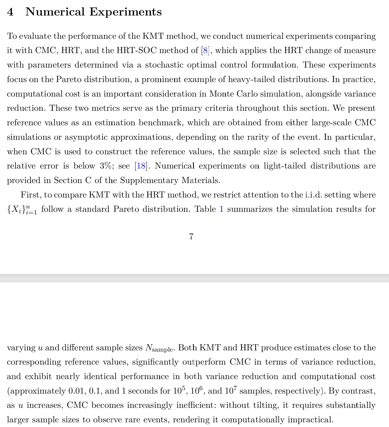
Figure 1 sets out the numerical experiments those claims rest on.
Figure 1: Liu et al (2026), Section 4, the numerical experiments.
2 What is reproducible
Unlike Ben Amar et al. (2023), this paper reports the probabilities, and it is careful about where its reference values come from. That makes it the best reproduction target of the group. Table 1 is the inventory.
Table 1: Every published value this page reproduces, its setting and where the paper’s reference comes from.
The Table C.1 references are exact in closed form, and the Table 2 reference at \(u = 444000\) is an analytic asymptotic. Both are checked independently in Table 3 before any of them is used to judge aggregate.
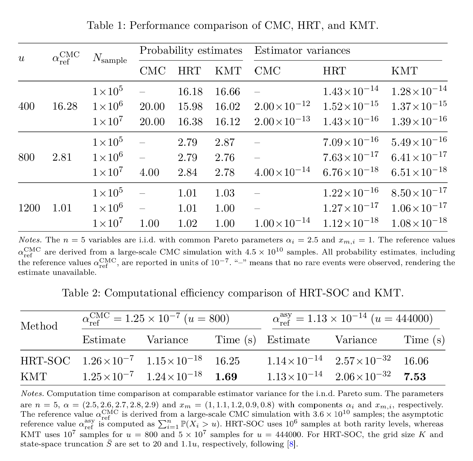
The estimator variances and CPU timings in all three published tables measure KMT and are not reproducible here, nor should they be. Figure 2 and Figure 4 are the pages they appear on.
Figure 2: Liu et al (2026), Tables 1 and 2.
3 Setup, and one parameterization trap
%xmode minimalimport warningsimport numpy as npimport pandas as pdfrom functools import partialfrom bookstyle import GT, build# Tail probabilities and relative errors read as powers of ten, not SI prefixes.GT = partial(GT, eng_style='exp')from scipy.integrate import IntegrationWarning# The Type I Paretos below have alpha near 2.5, so the tail integrals aggregate# evaluates for the severity moments really are slowly convergent and scipy says# so, 39 times. The warning is expected here and carries no information, and# because it prints an absolute path it also overflows the pdf text block by# 255pt each time. Filtered by category rather than blanket-suppressed, so any# other warning from this chapter still shows.warnings.filterwarnings('ignore', category=IntegrationWarning)ALPHAS = [2.5, 2.6, 2.7, 2.8, 2.9]XM = [1.0, 1.1, 1.2, 0.9, 0.8]LAM = [1.0, 1.2, 1.4, 1.5, 1.8]
so \(x_{m,i}\) enters as a scale, not as a location shift. This is the one place a reproduction silently goes wrong. In DecL, sev pareto 2.5 is scipy.stats.pareto(2.5) with unit scale, giving support \([1, \infty)\) and mean \(\alpha/(\alpha-1)\). To move the support to \([x_m, \infty)\) with the paper’s shape you must write sev {xm} * pareto {alpha}. Writing sev pareto {alpha} + {xm - 1} also puts the support in the right place but produces a shifted Pareto with a different tail, and the resulting probabilities are low by a few percent. Table 2 pins the convention on the severity means.
Table 2: Three Pareto severities written as scale times shape, each mean against the paper’s \(\alpha x_m/(\alpha-1)\).
DecL
agg mean
paper mean, a xm/(a-1)
sev 1 * pareto 2.5
1.667
1.667
sev 1.1 * pareto 2.6
1.788
1.788
sev 1.2 * pareto 2.7
1.906
1.906
Before trusting the paper’s own reference values, Table 3 checks the three that are analytic.
def asymptotic(u):"""Sum_i P(X_i > u) for Type I Pareto: the Table 2 reference at u=444000."""returnsum((x / u) ** a for a, x inzip(ALPHAS, XM))def hypoexponential_sf(t, lam):"""Exact survival of a sum of independent exponentials with distinct rates.""" lam = np.asarray(lam)returnsum(np.prod(np.delete(lam, i) / (np.delete(lam, i) - li)) * np.exp(-li * t)for i, li inenumerate(lam))GT(pd.DataFrame([ {'quantity': 'Table 2, u=444000', 'recomputed': asymptotic(444000.0),'paper': 1.13e-14}, {'quantity': 'Table C.1, u=25', 'recomputed': hypoexponential_sf(25.0-sum(XM), LAM),'paper': 2.73e-7}, {'quantity': 'Table C.1, u=28', 'recomputed': hypoexponential_sf(28.0-sum(XM), LAM),'paper': 1.40e-8},]))
Table 3: The Table 2 asymptotic and the two exact Table C.1 references, recomputed from their closed forms.
quantity
recomputed
paper
Table 2, u=444000
11.331e-15
11.300e-15
Table C.1, u=25
272.986e-09
273.000e-09
Table C.1, u=28
14.014e-09
14.000e-09
All three reproduce to the quoted precision in Table 3, which confirms the Type I reading and the shift convention \(X_i = Y_i + x_{m,i}\) in the light-tailed case.
4 Table 1: i.i.d. Pareto
Five i.i.d. Pareto variables is dfreq [5] against a single severity, and Table 4 is the result.
iid = build('agg T dfreq [5] sev 1 * pareto 2.5', log2=22, bs=1/16, padding=1, normalize=False)rows = []for u, ref, kmt in [(400, 1.628e-6, 1.612e-6), (800, 2.81e-7, 2.78e-7), (1200, 1.01e-7, 1.00e-7)]: s = iid.density_df.loc[u, 'S'] rows.append({'u': u, 'agg': s, 'paper CMC reference': ref,'rel err vs reference': abs(s / ref -1),'KMT at 1e7 samples': kmt})GT(pd.DataFrame(rows))
Table 4: Table 1, the i.i.d. Pareto tail probability at three thresholds, against the paper’s Monte Carlo reference and its KMT estimate.
u
agg
paper CMC reference
rel err vs reference
KMT at 1e7 samples
400
1.630e-06
1.628e-06
9.87e-04
1.612e-06
800
282.041e-09
281.000e-09
3.70e-03
278.000e-09
1,200
101.636e-09
101.000e-09
6.30e-03
100.000e-09
Table 4 agrees to between 0.1% and 0.6%. The reference itself comes from \(4.5 \times 10^{10}\) CMC samples, whose own relative standard error at \(\alpha \approx 10^{-7}\) is about 0.5%, so aggregate is inside the reference’s precision at every threshold and is at least as accurate as the KMT column at \(10^7\) samples.
The estimator variances in Table 1 are not reproducible, but they are still usable: they turn the paper into the formal acceptance test of Table 5. If aggregate is right, it should fall inside the KMT estimator’s own confidence interval.
kmt = [(400, 1.612e-6, 1.39e-16), (800, 2.78e-7, 6.51e-18), (1200, 1.00e-7, 1.08e-18)] # estimate and variance at 1e7 samplesrows = []for u, est, var in kmt: sd = var **0.5 s = iid.density_df.loc[u, 'S'] rows.append({'u': u, 'KMT estimate': est, 'KMT sd': sd,'lower 3 sd': est -3* sd, 'agg': s, 'upper 3 sd': est +3* sd,'z score': (s - est) / sd,'inside': abs(s - est) <3* sd})GT(pd.DataFrame(rows))
Table 5: The computed probability against a three standard error band around each KMT estimate.
u
KMT estimate
KMT sd
lower 3 sd
agg
upper 3 sd
z score
inside
400
1.612e-06
11.790e-09
1.577e-06
1.630e-06
1.647e-06
1.493
True
800
278.000e-09
2.551e-09
270.346e-09
282.041e-09
285.654e-09
1.584
True
1,200
100.000e-09
1.039e-09
96.882e-09
101.636e-09
103.118e-09
1.574
True
In Table 5aggregate sits within 1.6 standard errors of the KMT estimate at all three thresholds, which is what an unbiased estimator and an exact computation should do relative to one another. The \(z\) scores are notably consistent, all near \(+1.5\), which would suggest a small downward bias in the tabulated \(10^7\)-sample estimates if it were not for the fact that three points is too few to say so, and nothing in the paper indicates whether the three rows come from independent runs.
5 Table 2: i.n.d. Pareto, and where this stops working
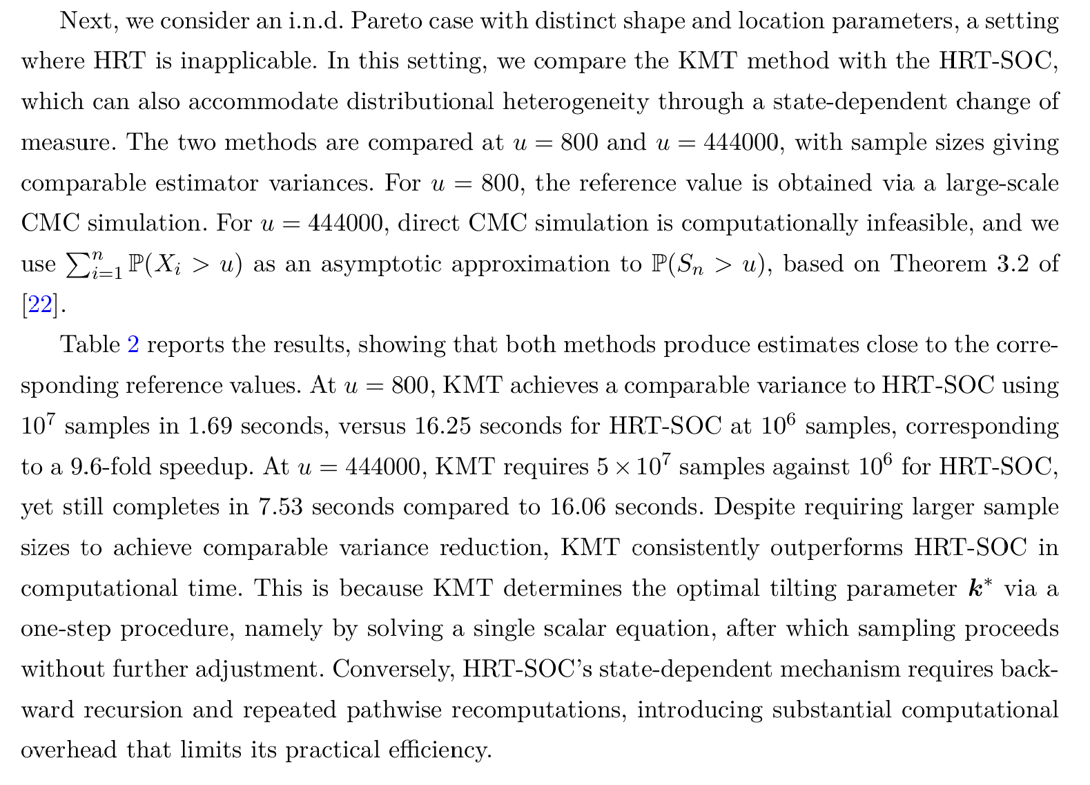
Distinct shapes and locations means a port of five one-claim aggregates. Figure 3 is the paper’s comparison against HRT-SOC and Table 6 the reproduction.
Figure 3: Liu et al (2026), the i.n.d. comparison against HRT-SOC.
units ='\n'.join(f'\tagg P{i} dfreq [1] sev {x} * pareto {al}'for i, (al, x) inenumerate(zip(ALPHAS, XM)))ind = build('port Paretos hints{log2=22;bs=1/8;padding=1;normalize=False}\n'+ units)rows = []for u, ref, kind in [(800, 1.25e-7, 'CMC, 3.6e10 samples'), (444000, 1.13e-14, 'asymptotic')]: s = ind.density_df.loc[u, 'S'] rows.append({'u': u, 'agg': s, 'paper reference': ref,'reference kind': kind, 'ratio agg / reference': s / ref})GT(pd.DataFrame(rows))
Table 6: Table 2, the i.n.d. Pareto tail probability at two thresholds, against a Monte Carlo and an asymptotic reference.
u
agg
paper reference
reference kind
ratio agg / reference
800
125.284e-09
125.000e-09
CMC, 3.6e10 samples
1.00
444,000
17.504e-12
11.300e-15
asymptotic
1,549.07
The \(u = 800\) row of Table 6 lands at 0.2%, against a reference built from \(3.6 \times 10^{10}\) Monte Carlo samples.
The \(u = 444000\) row is wrong by a factor of about 1550, and it is worth being precise about why, because the reason is not the model and not the parameterization. It is accumulated FFT roundoff. aggregate forms \(S(u)\) by summing bucket masses above \(u\), each carrying a rounding error of order machine epsilon times the local scale. Those errors are individually negligible and do not cancel, so the total scales with the number of buckets summed. At bs = 1/8 there are 642,304 buckets above 444000 and the accumulated bias swamps a \(10^{-14}\) answer.
That diagnosis makes a testable prediction: coarsen the grid, sum fewer buckets, and the answer should come back. Table 7 runs it.
rows = []for bs, log2 in [(1/8, 22), (1.0, 20), (8.0, 18), (64.0, 16), (512.0, 13), (4096.0, 10)]: p = build(f'port P hints{{log2={log2};bs={bs};padding=1;normalize=False}}\n'+ units) xs = p.density_df.index.values i = np.searchsorted(xs, 444000.0) s =float(p.density_df['S'].iloc[i]) rows.append({'bs': bs, 'log2': log2, 'x_max': xs[-1],'buckets above u': len(xs) - i, 'agg S(444000)': s,'ratio to reference': s / asymptotic(444000.0)})GT(pd.DataFrame(rows))
Table 7: The \(u = 444000\) probability as the grid is coarsened, against the number of buckets summed above the threshold.
bs
log2
x_max
buckets above u
agg S(444000)
ratio to reference
0.12
22
524.288e+03
642,304
17.504e-12
1,544.84
1.00
20
1.049e+06
604,576
3.933e-12
347.09
8.00
18
2.097e+06
206,644
883.404e-15
77.96
64.00
16
4.194e+06
58,598
197.287e-15
17.41
512.00
13
4.194e+06
7,324
44.853e-15
3.96
4,096.00
10
4.190e+06
915
11.324e-15
1.00
Table 7 behaves exactly as predicted, and monotonically. From 642,304 buckets down to 915, the ratio falls from 1545 to 1.01. At bs = 4096 the computed value is \(1.1435 \times 10^{-14}\) against the asymptotic reference \(1.1331 \times 10^{-14}\), a 0.9% agreement, and the small remaining excess is the genuine difference between the exact probability and the first-order asymptotic, which should be positive.
The practical lesson is counterintuitive and worth stating plainly: for a very small right-tail probability, coarsen the grid. Fine buckets buy resolution you do not need and pay for it in accumulated noise you cannot afford. This is the same absolute error floor documented on the Ben Rached et al. (2024) and Wilson and Keich (2017) pages, in a third guise: there it capped the depth of a left tail, here it caps the depth of a right tail, and in both cases it is proportional to how much of the density gets summed.
6 Table C.1: light-tailed, against an exact reference
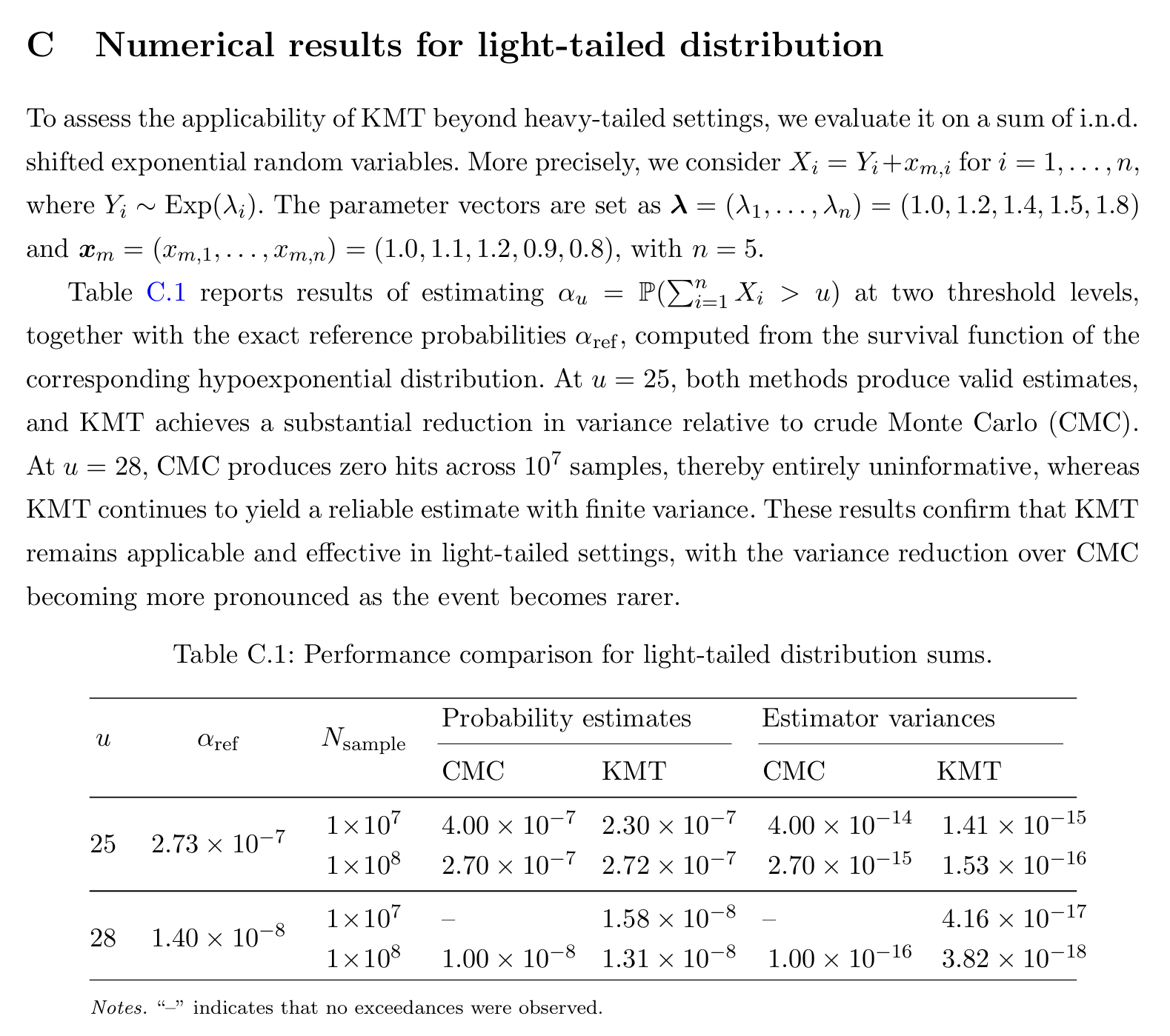
Figure 4: Liu et al (2026), Section C, light-tailed results.
Here \(X_i = Y_i + x_{m,i}\) with \(Y_i \sim \mathrm{Exp}(\lambda_i)\), so the shift genuinely is a shift and DecL’s + is correct. The reference is exact, which makes Table 8 the sharpest comparison in the paper.
Table 8: Table C.1, the light-tailed tail probability at two thresholds, against the exact hypoexponential value.
u
exact
agg
agg rel err
KMT 1e7
KMT 1e7 rel err
KMT 1e8
KMT 1e8 rel err
25
272.986e-09
272.855e-09
4.81e-04
230.000e-09
1.57e-01
272.000e-09
3.61e-03
28
14.014e-09
14.008e-09
4.84e-04
15.800e-09
1.27e-01
13.100e-09
6.53e-02
aggregate matches the exact value to about \(5 \times 10^{-4}\) at both thresholds. For comparison, KMT at \(10^8\) samples is 0.4% off at \(u = 25\) and 6.5% off at \(u = 28\), and at \(10^7\) samples it is 16% and 13% off. On this problem one deterministic build is between one and two orders of magnitude more accurate than \(10^8\) importance samples, and the gap widens as the event gets rarer, which is the opposite of how a sampler behaves.
That is not a criticism of KMT, whose target is generality rather than precision on a five-variable convolution. It is a statement about which tool fits this particular question.
7 Discussion
Three of the paper’s four reference points reproduce cleanly, two of them against references the paper itself derived analytically rather than by simulation. The fourth, \(u = 444000\), exceeds what a double precision FFT can deliver at a fine grid, and the grid study locates that boundary precisely rather than leaving it as a caveat.
The comparison worth drawing is with Ben Amar et al. (2023), reproduced on its own page. That paper reported no probabilities at all, only sample counts and CPU seconds, and the seven usable numbers had to be dug out of prose. This one tabulates the estimates, states the provenance of every reference, and gives exact references where exact references exist. The result is that it can be checked, and it checks out. Papers that report what they computed are more useful than papers that report only how fast they computed it, and this is a clean illustration.
On the substance, KMT looks right for what it claims. The power tilt is the natural move for a distribution with no moment generating function, minimizing a deterministic upper bound instead of the second moment is the standard tractable surrogate, and the threshold \(u_0\) characterizing where tilting starts to help is a genuinely useful practical output that most rare-event papers do not provide. The honest limitation, which the authors state, is independence: the whole construction is a product of marginal tilts, and dependence is listed as future work.
For the library, the note to carry forward is the parameterization trap and the grid lesson. Type I Pareto takes \(x_m\) as a scale, sev {xm} * pareto {alpha}, and getting that wrong costs a few percent in a way that shrinks with \(u\) and so looks like a convergence issue rather than a specification error. And when the target probability approaches \(10^{-13}\), the question to ask is not whether the grid is fine enough but whether it is too fine.
Programs in the aggregate Loss Lab
Each program below opens in the aggregate Loss Lab, which builds it with nothing to install. The names are those in reproductions.agg, where every program is renamed by its paper’s citation key.
Liu2026.T: a Pareto claim used in the k-moment tilting comparison.
Liu2026.T.v3: a Pareto claim used in the k-moment tilting comparison.
Liu2026.T.v4: a Pareto claim used in the k-moment tilting comparison.
Liu2026.T.v2: a Pareto claim used in the k-moment tilting comparison.
Liu2026.Paretos: Table 2's portfolio of non-identically distributed Paretos.
Liu2026.P: the same portfolio rebuilt across the grid sweep.
Liu2026.LT: Table C.1's light tailed portfolio, against an exact reference.
Ben Amar, E., Ben Rached, N., Haji-Ali, A.-L., & Tempone, R. (2023). State-dependent importance sampling for estimating expectations of functionals of sums of independent random variables. Statistics and Computing. https://doi.org/10.1007/s11222-022-10202-2
Ben Rached, N., Hoel, H., & Meo, J. V. (2024). A fast and accurate numerical method for the left tail of sums of independent random variables. Statistics and Computing. https://doi.org/10.1007/s11222-024-10514-5
Liu, Z., Wu, J., & Yao, J. (2026). Estimating tail probabilities of heavy-tailed distributions using k-moment tilting. Operations Research Letters. https://doi.org/10.1016/j.orl.2026.107509
Wilson, H., & Keich, U. (2017). Accurate small tail probabilities of sums of iid lattice-valued random variables via FFT. Journal of Computational and Graphical Statistics, 26(1), 223–229.