when the aggregate \(S\) is compound Poisson with a continuous severity. In 1982 the obstacle was that the recursion available at the time, Panjer’s, needs an arithmetic severity, so the continuous severity has to be discretized onto a span \(h\) first, and the discretization changes the answer.
The paper’s contribution is to bracket the error rather than hope about it. It sets out three ways to put a continuous severity onto a lattice of span \(h\):
move all the mass in a cell to its lower endpoint, which makes the aggregate smaller in the relevant order and produces a lower bound on the stop loss premium,
move it to the upper endpoint, giving an upper bound,
split the mass between the two endpoints so that the cell’s mean is preserved, the method of matching moments.
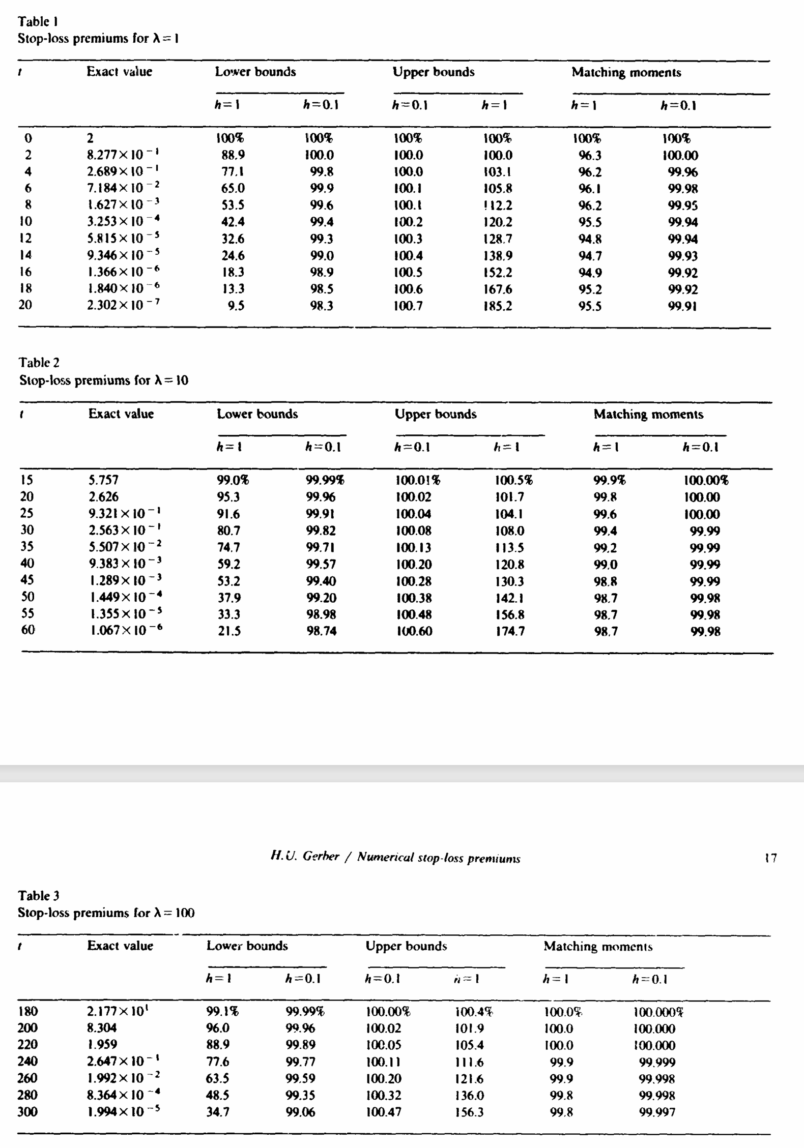
Tables 1 to 6 then show all three at \(h = 1\) and \(h = 0.1\) against an exact column, for expected claim counts 1, 10 and 100. The paper’s conclusion is that the bounds do bracket, that the upper bound is the better of the two, and that matching moments beats both by a wide margin: at \(\lambda = 100\) it does as well at \(h = 1\) as the bounds do at \(h = 0.1\).
Forty years later the interesting content is not the ranking, which is settled, but the exact column. It is 28 published four figure numbers for a compound Poisson with a continuous severity, computed by somebody with no FFT, and that makes it a good external check.
2 Paper solution and gold standard
Frequency is Poisson with mean \(\lambda\) and severity is uniform on \((1, 3)\), so \(\mathsf E[X] = 2\) and \(\mathsf E[S] = 2\lambda\). Tables 1, 2 and 3, Figure 1, tabulate \(\pi(t)\) for \(\lambda = 1, 10, 100\) at the retentions Table 1 lists.
The exact column is not a closed form. It is the paper’s own method (c) at \(h = 0.01\), and the paper says so: “column 2 gives the ‘exact’ stop-loss premium as calculated by method (c) with \(h = 0.01\). (A comparison with the results of methods (a) and (b) with \(h = 0.01\) has convinced the author that the displayed digits are accurate.)” So the target is four significant figures, and the reproduction is a comparison of two independent approximations rather than a check against truth.
Table 1: The three published tables, their claim counts and the retentions each tabulates.
table
lambda
E[S]
retentions
values
1
1
2
0 to 20
11
2
10
20
15 to 60
10
3
100
200
180 to 300
7
The severity supplies an acceptance test before any aggregate is built. A uniform on \((1, 3)\) has mean 2 and variance \(4/12 = 1/3\), so \(\mathsf E[S] = 2\lambda\) and \(\mathsf{Var}[S] = \lambda\,\mathsf E[X^2] = \lambda(4 + 1/3)\) by the compound Poisson variance formula. Table 2 records the two severity moments the check uses.
Table 2: The first two moments of the uniform severity on \((1, 3)\).
quantity
exact
severity mean
2.00000000
severity second moment
4.33333333
3 The aggregate reproduction
The severity is sev 2 * uniform + 1: a standard uniform scaled to width 2 and shifted to start at 1. Nothing else in the declaration varies across the three tables except \(\lambda\) and the grid, and Table 3 confirms all three builds before any premium is read.
Table 5: How many values reproduce inside the four significant figures the paper prints, table by table.
lambda
values compared
worst relative error
inside 4 significant figures
1
11
2.58e-04
11
10
10
3.53e-04
10
100
7
1.45e-04
7
all
28
3.53e-04
28
By Table 5 all 28 published values reproduce inside the four significant figures the paper prints, over a range of \(\pi(t)\) spanning eight orders of magnitude, from 21.77 down to \(2\times10^{-7}\). Two independent approximations to the same quantity, forty years apart, agree everywhere they can be compared.
4 Comments
4.1 The grid, and a correction to an earlier treatment
The bucket sizes above are not the obvious ones, and the \(\lambda = 100\) table is the reason. An earlier treatment of these tables in the technical guides used bs = 1/16 for \(\lambda = 100\), which is ample for the body and not for the tail, as Table 6 shows.
sweep = []for bs in (1/16, 1/64, 1/256): got = stop_loss(100, bs)for t, exact in PAPER[100].items(): sweep.append({'t': t, 'bs': f'1/{int(1/bs)}','rel err': abs(got[t] / exact -1)})piv = pd.DataFrame(sweep).pivot(index='t', columns='bs', values='rel err')piv = piv[[f'1/{d}'for d in (16, 64, 256)]]GT(piv, formatters={c: '{x:.2e}'for c in piv.columns})
Table 6: Relative error on Table 3 at three bucket sizes, showing where the coarse grid fails.
t
1/16
1/64
1/256
180
1.61e-04
1.45e-04
1.44e-04
200
1.27e-04
5.76e-05
5.32e-05
220
2.61e-04
6.48e-05
5.25e-05
240
4.23e-04
4.41e-06
2.17e-05
260
6.95e-04
4.91e-05
9.56e-05
280
1.31e-03
1.28e-04
5.44e-05
300
1.60e-03
1.15e-04
2.23e-04
In Table 6, at bs = 1/16 the last three rows of Table 3 miss the printed precision, by up to \(1.6\times10^{-3}\) at \(t = 300\). Refining to bs = 1/64 brings every row inside \(2\times10^{-4}\) and refining again changes little, so the residual was discretization on this side and not an inaccuracy in Gerber’s column. That is worth stating the right way round: the first version of this comparison looked like a small failure of the paper’s far tail digits, and it was not.
The general point is the one Mack and Fackler (2003) makes from a different direction. A grid sized for the mean is not automatically a grid sized for a tail eight orders of magnitude down, and the quantity that reveals it is the one being read, not the mean or the total mass, both of which are already exact to twelve figures at bs = 1/16.
4.2 What became of the three methods
Gerber’s three discretizations are still the live choices, and aggregate exposes the same distinction as discretization_calc, which computes the discrete probabilities from the survival function or the distribution function and so is accurate on the right or the left tail. The library’s default is the moment preserving idea rather than either bound, which is Gerber’s method (c) and his own recommendation.
What has changed is that the bound is no longer the thing you reach for. Gerber needed bounds because his exact answer cost as much as the bracket did, so bracketing was the cheap way to know he was close. Here the fine grid is the cheap option: the whole of Table 3 at bs = 1/256 costs a fraction of a second, so the honest error control is refinement and comparison, and this page uses it above rather than a bound.
4.3 Why a uniform severity is a good test and a bad model
Uniform on \((1, 3)\) is not a claim size distribution anybody would fit. It is a deliberately awkward test case, and the awkward part is the two hard edges. A severity with compact support and a discontinuous density at both ends is the worst case for any discretization scheme, because the error does not smooth out across a cell boundary the way it does for a density that decays. That the reproduction holds to four figures on a severity chosen to be difficult, rather than on a lognormal, says more than the same result on a friendly curve would.
It also has an exact aggregate at small \(\lambda\), which is how the \(t = 0\) row can be checked to twelve figures: \(\pi(0) = \mathsf E[S] = 2\lambda\) with no discretization involved at all.
Programs in the aggregate Loss Lab
Each program below opens in the aggregate Loss Lab, which builds it with nothing to install. The names are those in reproductions.agg, where every program is renamed by its paper’s citation key.
Gerber1982.Gerber: a compound Poisson on a uniform severity, for the stop loss table.
Gerber1982.Gerber.v2: a compound Poisson on a uniform severity, for the stop loss table.
Gerber1982.Gerber.v3: a compound Poisson on a uniform severity, for the stop loss table.
Gerber, H. U. (1982). On the numerical evaluation of the distribution of aggregate claims and its stop-loss premiums. Insurance Mathematics and Economics, 1(1), 13–18. https://doi.org/10.1016/0167-6687(82)90016-6
Mack, T., & Fackler, M. (2003). Exposure-rating in liability reinsurance. Blätter der DGVFM, 26(2), 229–238.
4 Comments
4.1 The grid, and a correction to an earlier treatment
The bucket sizes above are not the obvious ones, and the \(\lambda = 100\) table is the reason. An earlier treatment of these tables in the technical guides used
bs = 1/16for \(\lambda = 100\), which is ample for the body and not for the tail, as Table 6 shows.In Table 6, at
bs = 1/16the last three rows of Table 3 miss the printed precision, by up to \(1.6\times10^{-3}\) at \(t = 300\). Refining tobs = 1/64brings every row inside \(2\times10^{-4}\) and refining again changes little, so the residual was discretization on this side and not an inaccuracy in Gerber’s column. That is worth stating the right way round: the first version of this comparison looked like a small failure of the paper’s far tail digits, and it was not.The general point is the one Mack and Fackler (2003) makes from a different direction. A grid sized for the mean is not automatically a grid sized for a tail eight orders of magnitude down, and the quantity that reveals it is the one being read, not the mean or the total mass, both of which are already exact to twelve figures at
bs = 1/16.4.2 What became of the three methods
Gerber’s three discretizations are still the live choices, and
aggregateexposes the same distinction asdiscretization_calc, which computes the discrete probabilities from the survival function or the distribution function and so is accurate on the right or the left tail. The library’s default is the moment preserving idea rather than either bound, which is Gerber’s method (c) and his own recommendation.What has changed is that the bound is no longer the thing you reach for. Gerber needed bounds because his exact answer cost as much as the bracket did, so bracketing was the cheap way to know he was close. Here the fine grid is the cheap option: the whole of Table 3 at
bs = 1/256costs a fraction of a second, so the honest error control is refinement and comparison, and this page uses it above rather than a bound.4.3 Why a uniform severity is a good test and a bad model
Uniform on \((1, 3)\) is not a claim size distribution anybody would fit. It is a deliberately awkward test case, and the awkward part is the two hard edges. A severity with compact support and a discontinuous density at both ends is the worst case for any discretization scheme, because the error does not smooth out across a cell boundary the way it does for a density that decays. That the reproduction holds to four figures on a severity chosen to be difficult, rather than on a lognormal, says more than the same result on a friendly curve would.
It also has an exact aggregate at small \(\lambda\), which is how the \(t = 0\) row can be checked to twelve figures: \(\pi(0) = \mathsf E[S] = 2\lambda\) with no discretization involved at all.