Homer and Clark’s bivariate FFT

Reproducing Homer and Clark (2003)

1 Context and problem

The collective risk model gives the distribution of a sum of claims. It does not, on its own, give the joint distribution of two quantities that both depend on the same claims. Homer and Clark (2003) gives three examples where the joint distribution is needed.

1. An insured retains the first $600,000 of each occurrence and buys a stop loss on the total retention. The insurer thus writes two covers: a per occurrence excess of $600,000 and an aggregate stop loss on the retention, a “specific and agg”. It can price either cover alone, but not their sum, because the two are dependent: an excess loss can only happen if the retention was breached.
2. A general liability policy caps indemnity but pays defense costs in addition, so the aggregate is loss capped at a policy aggregate plus uncapped expense, with the two correlated at the claim level.
3. A dynamic financial analysis model simulates small losses in aggregate and large losses individually, and treating them as independent understates the tail, because a high claim count raises both.

Their answer is the 2-d analog of our standard FFT-convolution algorithm: build a bivariate per-claim severity matrix \(M_x\) whose \((j,k)\) entry is the joint probability of the two components, then \[ M_z = \mathrm{IFFT}\left(\mathrm{PGF}\left(\mathrm{FFT}(M_x)\right)\right) \] with a two-dimensional transform and the claim count probability generating function applied elementwise. The frequency couples the two axes; the severity matrix carries the per-claim dependence; and one transform delivers the joint aggregate.

Mildenhall (2005) describes a second approach with a bivariate frequency distribution, but that is not considered here.

2 Paper solution and gold standard

The paper provides three fully specified examples, each with the input and output matrices, as Table 1 sets out.

Table 1: The three worked examples, their axes, their frequencies and what each publishes.

Section	Axes	Frequency	Published
2	retained loss, excess loss	NB mean 5, variance 6	Tables 2.3 to 2.6 plus five statistics
3	indemnity loss, ALAE	NB mean 4, variance 8	Tables 3.3 to 3.6
4	small loss dollars, large loss counts	NB mean 10, variance 20	Tables 4.2 to 4.4

Appendix A provides an R code doing a \(3\times3\) two-dimensional FFT by hand, and Appendix B derives a closed-form covariance between small and large aggregate losses. Both are checkable.

The negative binomial enters through its probability generating function, which the paper writes in terms of mean \(M\) and variance \(V\) as \[ \phi(t) = (V/M - (V/M - 1)t)^{-M^2/(V-M)}. \] Note that for over-dispersed distributions \(V>M\), with the Poisson lower limit \(V=M\). aggregate describes the same law as a gamma-mixed Poisson: matching \(n + n^2c^2 = V\) at \(n = M\) gives mixing coefficient of variation \[ c = \sqrt{(V-M)/M^2} = \sqrt{(\nu-1)/n} \] where \(\nu=V/M\) is the variance-to-mean ratio. Table 2 translates the paper’s three probability generating functions into the mixing CV each build needs.

%xmode minimal
import numpy as np
import pandas as pd
from bookstyle import GT, build

K = 200_000.0

def nb_cv(mean, var):
    """Gamma mixing CV reproducing a negative binomial with this mean and variance."""
    return float(np.sqrt((var - mean) / mean ** 2))

GT(pd.DataFrame([
    {'section': 2, 'NB mean': 5, 'NB variance': 6, 'paper PGF': '$(1.2 - 0.2t)^{-25}$',
     'mixed gamma cv': nb_cv(5, 6)},
    {'section': 3, 'NB mean': 4, 'NB variance': 8, 'paper PGF': '$(2 - t)^{-4}$',
     'mixed gamma cv': nb_cv(4, 8)},
    {'section': 4, 'NB mean': 10, 'NB variance': 20, 'paper PGF': '$(2 - t)^{-10}$',
     'mixed gamma cv': nb_cv(10, 20)},
]))

Exception reporting mode: Minimal

Table 2: The paper’s three negative binomial frequencies, and the gamma mixing CV that reproduces each.

section	NB mean	NB variance	paper PGF	mixed gamma cv
2	5	6	\((1.2 - 0.2t)^{-25}\)	0.20000
3	4	8	\((2 - t)^{-4}\)	0.50000
4	10	20	\((2 - t)^{-10}\)	0.31623

Before introducing the insurance examples, we provide an arithmetic check. Appendix A convolves \[ M_x = \begin{pmatrix}.4 & 0 & 0\\ .3 & .3 & 0\\ 0&0&0\end{pmatrix} \] with itself and prints the answer. In DecL that is a fixed count of two against a discrete bivariate severity, computed in Table 3.

toy = build('bivariate A dfreq [2] dbvsev [0 1 2] [0 1 2] '
            '[[.4 0 0] [.3 .3 0] [0 0 0]]', bs=(1., 1.), log2=(3, 3))
GT(pd.DataFrame(toy.density[:3, :3], index=[0, 1, 2], columns=[0, 1, 2]),
   float_format=6)

Table 3: The Appendix A \(3\times3\) matrix convolved with itself.

level_0	0	1	2
0	0.160000	0.000000	0.000000
1	0.240000	0.240000	0.000000
2	0.090000	0.180000	0.090000

The paper’s R session returns 0.16, 0.24, 0.09 down the first column and 0.24, 0.18, 0.09 for the rest, which is what Table 3 came back with.

3 Section 2: Per-Occurrence And Stop Loss

Dietrichson Drilling retains $600,000 per occurrence and buys $400,000 xs $600,000 per occurrence plus $5,000,000 xs $3,000,000 on the aggregate retention. Severity is the five point discrete law of Figure 1; frequency is negative binomial with mean 5 and variance 6.

Figure 1: Homer and Clark (2003), Table 2.2.

The paper builds Table 2.3, Figure 2, the joint per-claim law of retained and ceded, by hand. aggregate does not need it built: retained and ceded are the net and ceded views of an occurrence layer, so the bivariate severity is the cession map applied to the gross severity. That is occ_bivariate, and the DecL keyword is netceded. The remaining targets for this section are Figure 3, Figure 4 and Figure 5.

Figure 2: Homer and Clark (2003), Table 2.3.

Figure 3: Homer and Clark (2003), Table 2.4.

Figure 4: Homer and Clark (2003), Table 2.5.

Figure 5: Homer and Clark (2003), Table 2.6.

Table 4 records the grid the build lands on and checks the severity mean against the paper’s.

SEV = 'dsev [200000 400000 600000 800000 1000000] [.378 .235 .146 .091 .15]'
a = build(f'agg HC 5 claims {SEV} occurrence net of 400000 xs 600000 '
          f'mixed gamma {nb_cv(5, 6)}', bs=K, log2=8)
bd = a.occ_bivariate(views=('net', 'ceded'), bs=K, log2_x=7, log2_y=5)
gx, gy = bd.axis_xs
d = bd.density
GT(pd.DataFrame([{'grid': str(d.shape), 'bs': str(bd.bs),
                  'deficit': bd.deficit, 'total mass': d.sum(),
                  'severity mean': (np.arange(5) + 1) @ np.array(
                      [.378, .235, .146, .091, .15]) * K,
                  'paper severity mean': 480_000}]))

Table 4: The section 2 bivariate grid, its mass deficit, and the severity mean against the paper’s $480,000.

grid	bs	deficit	total mass	severity mean	paper severity mean
(128, 32)	[200000.0, 200000.0]	93.703f	1.00000	480,000	480,000

The single claim joint law is a by-product, and it is Table 2.3: compare Table 5 with Figure 2.

S = np.asarray(bd._S.todense()) if hasattr(bd._S, 'todense') else bd._S
GT(pd.DataFrame(100 * S[:6, :4], index=[f'{v:,.0f}' for v in gx[:6]],
                columns=[f'{v:,.0f}' for v in gy[:4]]), float_format=2)

Table 5: The joint per-claim law of retained and ceded, as percentages, read off the cession map.

level_0	0	200,000	400,000	600,000
0	0.00	0.00	0	0
200,000	37.80	0.00	0	0
400,000	23.50	0.00	0	0
600,000	14.60	9.10	15	0
800,000	0.00	0.00	0	0
1,000,000	0.00	0.00	0	0

Table 2.4 is the aggregate joint. The paper prints a \(26\times7\) block of it to two decimals, reproduced in Table 6 and scored in Table 7.

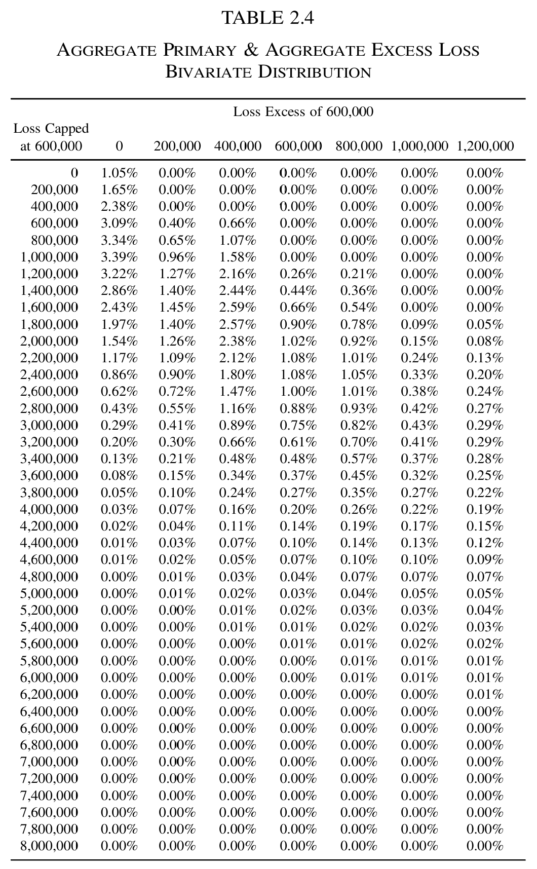
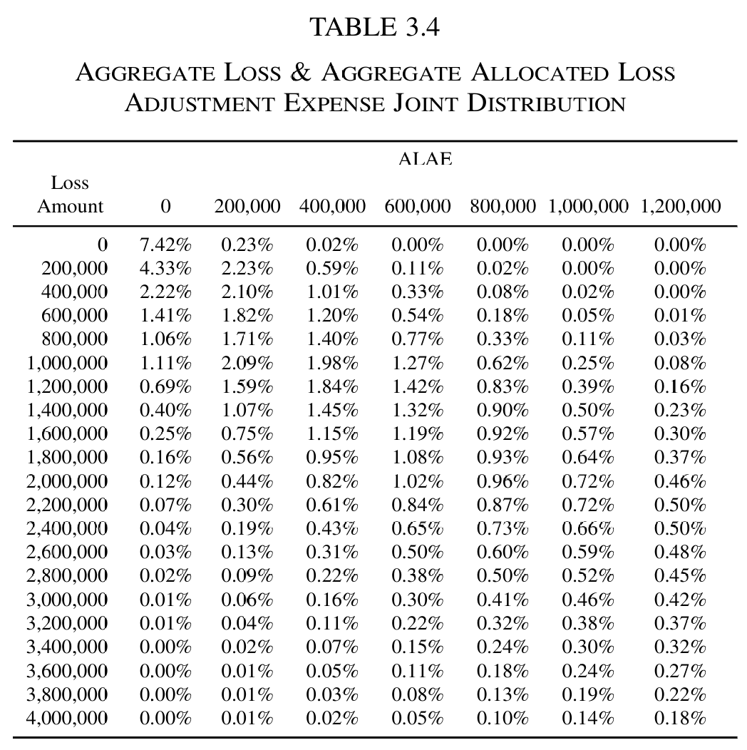
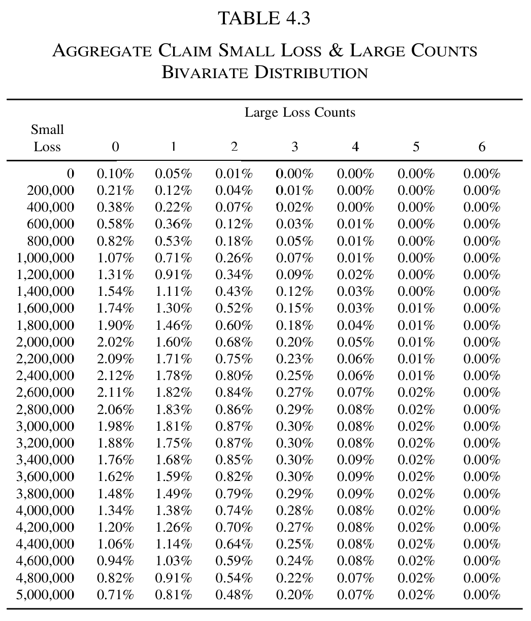
T24 = {0: [1.05, 0, 0, 0, 0, 0, 0], 200_000: [1.65, 0, 0, 0, 0, 0, 0],
       400_000: [2.38, 0, 0, 0, 0, 0, 0],
       600_000: [3.09, .40, .66, 0, 0, 0, 0],
       800_000: [3.34, .65, 1.07, 0, 0, 0, 0],
       1_000_000: [3.39, .96, 1.58, 0, 0, 0, 0],
       1_200_000: [3.22, 1.27, 2.16, .26, .21, 0, 0],
       1_400_000: [2.86, 1.40, 2.44, .44, .36, 0, 0],
       1_600_000: [2.43, 1.45, 2.59, .66, .54, 0, 0],
       1_800_000: [1.97, 1.40, 2.57, .90, .78, .09, .05],
       2_000_000: [1.54, 1.26, 2.38, 1.02, .92, .15, .08],
       2_200_000: [1.17, 1.09, 2.12, 1.08, 1.01, .24, .13],
       2_400_000: [.86, .90, 1.80, 1.08, 1.05, .33, .20],
       2_600_000: [.62, .72, 1.47, 1.00, 1.01, .38, .24],
       2_800_000: [.43, .55, 1.16, .88, .93, .42, .27],
       3_000_000: [.29, .41, .89, .75, .82, .43, .29],
       3_200_000: [.20, .30, .66, .61, .70, .41, .29],
       3_400_000: [.13, .21, .48, .48, .57, .37, .28],
       3_600_000: [.08, .15, .34, .37, .45, .32, .25],
       3_800_000: [.05, .10, .24, .27, .35, .27, .22],
       4_000_000: [.03, .07, .16, .20, .26, .22, .19],
       4_200_000: [.02, .04, .11, .14, .19, .17, .15],
       4_400_000: [.01, .03, .07, .10, .14, .13, .12],
       4_600_000: [.01, .02, .05, .07, .10, .10, .09],
       4_800_000: [0, .01, .03, .04, .07, .07, .07],
       5_000_000: [0, .01, .02, .03, .04, .05, .05]}
got24 = np.array([100 * d[int(round(r / K)), :7] for r in T24])
pap24 = np.array(list(T24.values()))
GT(pd.DataFrame(got24, index=[f'{r:,.0f}' for r in T24],
                columns=[f'{int(j * K):,.0f}' for j in range(7)]),
   float_format=2)

Table 6: The aggregate joint distribution of net and ceded, the \(26\times7\) block Table 2.4 prints, as percentages.

level_0	0	200,000	400,000	600,000	800,000	1,000,000	1,200,000
0	1.05	0.00	0.00	0.00	0.00	0.00	0.00
200,000	1.65	0.00	0.00	0.00	0.00	0.00	0.00
400,000	2.38	0.00	0.00	0.00	0.00	0.00	0.00
600,000	3.09	0.40	0.66	0.00	0.00	0.00	0.00
800,000	3.34	0.65	1.07	0.00	0.00	0.00	0.00
1,000,000	3.39	0.96	1.58	0.00	0.00	0.00	0.00
1,200,000	3.22	1.27	2.16	0.26	0.21	0.00	0.00
1,400,000	2.86	1.40	2.44	0.44	0.36	0.00	0.00
1,600,000	2.43	1.45	2.59	0.66	0.54	0.00	0.00
1,800,000	1.97	1.40	2.57	0.90	0.78	0.09	0.05
2,000,000	1.54	1.26	2.38	1.02	0.92	0.15	0.08
2,200,000	1.17	1.09	2.12	1.08	1.01	0.24	0.13
2,400,000	0.86	0.90	1.80	1.08	1.05	0.33	0.20
2,600,000	0.62	0.72	1.47	1.00	1.01	0.38	0.24
2,800,000	0.43	0.55	1.16	0.88	0.93	0.42	0.27
3,000,000	0.29	0.41	0.89	0.75	0.82	0.43	0.29
3,200,000	0.20	0.30	0.66	0.61	0.70	0.41	0.29
3,400,000	0.13	0.21	0.48	0.48	0.57	0.37	0.28
3,600,000	0.08	0.15	0.34	0.37	0.45	0.32	0.25
3,800,000	0.05	0.10	0.24	0.27	0.35	0.27	0.22
4,000,000	0.03	0.07	0.16	0.20	0.26	0.22	0.19
4,200,000	0.02	0.04	0.11	0.14	0.19	0.17	0.15
4,400,000	0.01	0.03	0.07	0.10	0.14	0.13	0.12
4,600,000	0.01	0.02	0.05	0.07	0.10	0.10	0.09
4,800,000	0.00	0.01	0.03	0.04	0.07	0.07	0.07
5,000,000	0.00	0.01	0.02	0.03	0.04	0.05	0.05

GT(pd.DataFrame([{'cells compared': got24.size,
                  'worst absolute difference, points of probability':
                      float(np.abs(got24 - pap24).max())}]))

Table 7: Worst cell error over the whole published block of Table 2.4.

cells compared	worst absolute difference, points of probability
182	0.00497

Table 2.5, Figure 4, applies the stop loss: collapse every net outcome at or below $3,000,000 into one row and relabel the rest. Then the five statistics the paper quotes fall straight out of the joint, in Table 8.

k = int(round(3_000_000 / K))
d25 = np.vstack([d[:k + 1].sum(axis=0)[None, :], d[k + 1:]])
g25 = np.arange(d25.shape[0]) * K
hit = 1 - d25.sum(axis=1)[0]
GT(pd.DataFrame([
    {'statistic': 'expected loss to the stop loss layer',
     'aggregate': (d25.sum(axis=1) * g25).sum(), 'paper': 123_529},
    {'statistic': 'probability the stop loss is hit',
     'aggregate': hit, 'paper': 0.1508},
    {'statistic': 'mean stop loss given it is hit',
     'aggregate': (d25[1:].sum(axis=1) * g25[1:]).sum() / hit, 'paper': 819_210},
    {'statistic': 'expected loss to the per-occurrence layer',
     'aggregate': (d25.sum(axis=0) * gy).sum(), 'paper': 391_000},
    {'statistic': 'expected per-occurrence loss given the stop loss is hit',
     'aggregate': (d25[1:].sum(axis=0) * gy).sum() / hit, 'paper': 830_334},
]), float_format=4)

Table 8: The five statistics the paper quotes off Table 2.5, taken from the joint distribution.

statistic	aggregate	paper
expected loss to the stop loss layer	123,529.2639	123,529.0000
probability the stop loss is hit	0.1508	0.1508
mean stop loss given it is hit	819,209.9260	819,210.0000
expected loss to the per-occurrence layer	391,000.0000	391,000.0000
expected per-occurrence loss given the stop loss is hit	830,334.0247	830,334.0000

Table 8 has all five to the digit. The last two are the paper’s punchline: the per-occurrence layer costs $391,000 on average, but $830,334 in the scenarios where the stop loss also pays. Writing both covers is more than twice as bad as the two expected values suggest, and that is invisible to anyone pricing the covers separately.

Table 2.6 sums the antidiagonals to get the distribution of the two covers combined, Table 9.

n = 5
tot = np.zeros(n)
for i in range(d25.shape[0]):
    for j in range(min(d25.shape[1], n)):
        if i + j < n:
            tot[i + j] += d25[i, j]
GT(pd.DataFrame({'combined loss': [f'{i * K:,.0f}' for i in range(n)],
                 'aggregate %': 100 * tot,
                 'Table 2.6 %': [30.28, 12.64, 23.31, 9.02, 8.94]}),
   float_format=2)

Table 9: The distribution of the two covers combined, against the five cells Table 2.6 prints.

combined loss	aggregate %	Table 2.6 %
0	30.28	30.28
200,000	12.64	12.64
400,000	23.31	23.31
600,000	9.02	9.02
800,000	8.94	8.94

4 Section 3: loss subject to an aggregate, plus unlimited ALAE

Here the bivariate severity is given rather than derived, so DecL takes the matrix directly with dbvsev.

Figure 6: Homer and Clark (2003), Table 3.2.

One transcription note. Table 3.3, Figure 7, is printed to two decimals and its row sums are 10.00%, 45.00%, 9.00%, 9.00%, 9.00% and 17.97%, against the loss marginal of Figure 6 which requires 18.00% on the last. The printed matrix therefore carries 99.97% of the mass. Scaling each row to its Table 3.2 marginal is the correction the paper’s own inputs dictate. The outputs to match are Figure 8, Figure 9 and Figure 10.

Figure 7: Homer and Clark (2003), Table 3.3.

Figure 8: Homer and Clark (2003), Table 3.4.

Figure 9: Homer and Clark (2003), Table 3.5.

Figure 10: Homer and Clark (2003), Table 3.6.

Table 10 records the grid and checks both marginal means, and Table 11 is the published block itself.

XS3 = [0, 200e3, 400e3, 600e3, 800e3, 1000e3]
YS3 = [0, 200e3, 400e3, 600e3, 800e3, 1000e3, 1200e3]
M3 = np.array([
    [.0839, .0147, .0013, .0001, .0000, .0000, .0000],
    [.2798, .1329, .0316, .0050, .0006, .0001, .0000],
    [.0415, .0321, .0125, .0032, .0006, .0001, .0000],
    [.0307, .0330, .0177, .0064, .0017, .0004, .0001],
    [.0228, .0313, .0215, .0099, .0034, .0009, .0002],
    [.0337, .0565, .0473, .0264, .0111, .0037, .0010]])
TARGET = np.array([.10, .45, .09, .09, .09, .18])       # Table 3.2
M3 = M3 * (TARGET / M3.sum(axis=1))[:, None]

def dbvsev(name, xs, ys, M, count, cv):
    rows = ' '.join('[' + ' '.join(f'{float(v):.12g}' for v in r) + ']'
                    for r in M)
    return (f'bivariate {name} {count} claims '
            f'dbvsev [{" ".join(f"{float(v):.0f}" for v in xs)}] '
            f'[{" ".join(f"{float(v):.0f}" for v in ys)}] [{rows}] '
            f'mixed gamma {cv}')

b3 = build(dbvsev('HC3', XS3, YS3, M3, 4, nb_cv(4, 8)), bs=(K, K), log2=(7, 6))
d3 = b3.density
GT(pd.DataFrame([{'grid': str(d3.shape), 'deficit': b3.deficit,
                  'loss mean': (d3.sum(axis=1) * b3.axis_xs[0]).sum(),
                  'paper 4 x 432,000': 4 * 432_000,
                  'ALAE mean': (d3.sum(axis=0) * b3.axis_xs[1]).sum()}]))

Table 10: The section 3 bivariate grid, its mass deficit, and the loss and ALAE means.

grid	deficit	loss mean	paper 4 x 432,000	ALAE mean
(128, 64)	1.906p	1.728M	1,728,000	656,960

T34 = {0: [7.42, .23, .02, 0, 0, 0, 0],
       200_000: [4.33, 2.23, .59, .11, .02, 0, 0],
       400_000: [2.22, 2.10, 1.01, .33, .08, .02, 0],
       600_000: [1.41, 1.82, 1.20, .54, .18, .05, .01],
       800_000: [1.06, 1.71, 1.40, .77, .33, .11, .03],
       1_000_000: [1.11, 2.09, 1.98, 1.27, .62, .25, .08],
       1_200_000: [.69, 1.59, 1.84, 1.42, .83, .39, .16],
       1_400_000: [.40, 1.07, 1.45, 1.32, .90, .50, .23],
       1_600_000: [.25, .75, 1.15, 1.19, .92, .57, .30],
       1_800_000: [.16, .56, .95, 1.08, .93, .64, .37],
       2_000_000: [.12, .44, .82, 1.02, .96, .72, .46],
       2_200_000: [.07, .30, .61, .84, .87, .72, .50],
       2_400_000: [.04, .19, .43, .65, .73, .66, .50],
       2_600_000: [.03, .13, .31, .50, .60, .59, .48],
       2_800_000: [.02, .09, .22, .38, .50, .52, .45],
       3_000_000: [.01, .06, .16, .30, .41, .46, .42],
       3_200_000: [.01, .04, .11, .22, .32, .38, .37],
       3_400_000: [0, .02, .07, .15, .24, .30, .32],
       3_600_000: [0, .01, .05, .11, .18, .24, .27],
       3_800_000: [0, .01, .03, .08, .13, .19, .22],
       4_000_000: [0, .01, .02, .05, .10, .14, .18]}
got34 = np.array([100 * d3[int(round(r / K)), :7] for r in T34])
GT(pd.DataFrame(got34, index=[f'{r:,.0f}' for r in T34],
                columns=[f'{int(j * K):,.0f}' for j in range(7)]),
   float_format=2)

Table 11: The aggregate joint distribution of capped loss and ALAE, the \(21\times7\) block Table 3.4 prints, as percentages.

level_0	0	200,000	400,000	600,000	800,000	1,000,000	1,200,000
0	7.42	0.23	0.02	0.00	0.00	0.00	0.00
200,000	4.33	2.22	0.59	0.11	0.02	0.00	0.00
400,000	2.22	2.10	1.01	0.33	0.08	0.02	0.00
600,000	1.41	1.82	1.20	0.54	0.18	0.05	0.01
800,000	1.06	1.70	1.39	0.77	0.33	0.11	0.03
1,000,000	1.11	2.09	1.98	1.27	0.62	0.25	0.08
1,200,000	0.69	1.59	1.84	1.42	0.84	0.40	0.16
1,400,000	0.40	1.07	1.45	1.32	0.90	0.50	0.23
1,600,000	0.25	0.75	1.15	1.19	0.92	0.57	0.30
1,800,000	0.17	0.56	0.95	1.08	0.93	0.64	0.37
2,000,000	0.12	0.44	0.82	1.02	0.96	0.72	0.46
2,200,000	0.07	0.30	0.62	0.84	0.87	0.72	0.50
2,400,000	0.04	0.19	0.43	0.65	0.73	0.66	0.50
2,600,000	0.03	0.13	0.31	0.50	0.61	0.59	0.48
2,800,000	0.02	0.09	0.22	0.38	0.50	0.52	0.46
3,000,000	0.01	0.06	0.16	0.30	0.41	0.46	0.42
3,200,000	0.01	0.04	0.11	0.22	0.32	0.38	0.38
3,400,000	0.00	0.02	0.07	0.15	0.24	0.30	0.32
3,600,000	0.00	0.01	0.05	0.11	0.18	0.24	0.27
3,800,000	0.00	0.01	0.03	0.08	0.13	0.19	0.22
4,000,000	0.00	0.01	0.02	0.05	0.10	0.15	0.18

CAP = 2_000_000
kc = int(round(CAP / K))
d35 = np.vstack([d3[:kc], d3[kc:].sum(axis=0)[None, :]])
n = 5
tot3 = np.zeros(n)
for i in range(d35.shape[0]):
    for j in range(min(d35.shape[1], n)):
        if i + j < n:
            tot3[i + j] += d35[i, j]
GT(pd.DataFrame([
    {'check': 'Table 3.4, worst of the 21 x 7 published cells, points',
     'value': float(np.abs(got34 - np.array(list(T34.values()))).max())},
    {'check': 'Table 3.6, worst of the 5 published cells, points',
     'value': float(np.abs(100 * tot3
                           - np.array([7.42, 4.56, 4.47, 4.09, 3.99])).max())},
]), float_format=4)

Table 12: Worst published cell error for Tables 3.4 and 3.6.

check	value
Table 3.4, worst of the 21 x 7 published cells, points	0.0061
Table 3.6, worst of the 5 published cells, points	0.0036

GT(pd.DataFrame({'loss (capped) + ALAE': [f'{i * K:,.0f}' for i in range(n)],
                 'aggregate %': 100 * tot3,
                 'Table 3.6 %': [7.42, 4.56, 4.47, 4.09, 3.99]}),
   float_format=2)

Table 13: Capped loss plus ALAE combined, against the five cells Table 3.6 prints.

loss (capped) + ALAE	aggregate %	Table 3.6 %
0	7.42	7.42
200,000	4.56	4.56
400,000	4.47	4.47
600,000	4.09	4.09
800,000	3.99	3.99

Table 12 scores both, and Table 13 prints the combined distribution itself. The $2,000,000 general aggregate applies to indemnity only, so the cap is a row collapse on the loss axis with the ALAE axis untouched. That asymmetry is the whole reason the example needs a joint distribution: cap the sum and you have the wrong contract.

5 Section 4: dollars against counts

The third example puts aggregate small loss dollars on one axis and large loss counts on the other. The bivariate severity is degenerate by construction: a claim is either small, contributing dollars and no count, or large, contributing one count and no dollars. The inputs are Figure 11 and Figure 12, and the targets Figure 13 and Figure 14.

Figure 11: Homer and Clark (2003), Table 4.1.

Figure 12: Homer and Clark (2003), Table 4.2.

Figure 13: Homer and Clark (2003), Table 4.3.

Figure 14: Homer and Clark (2003), Table 4.4.

XS4 = [0, 200e3, 400e3, 600e3, 800e3]
YS4 = [0, 1, 2, 3, 4, 5]
M4 = np.array([[.000, .100, 0, 0, 0, 0],
               [.438, .000, 0, 0, 0, 0],
               [.246, .000, 0, 0, 0, 0],
               [.138, .000, 0, 0, 0, 0],
               [.078, .000, 0, 0, 0, 0]])
b4 = build(dbvsev('HC4', XS4, YS4, M4, 10, nb_cv(10, 20)),
           bs=(K, 1.0), log2=(7, 5))
d4 = b4.density
gx4, gy4 = b4.axis_xs
T43 = {0: [.10, .05, .01, 0, 0, 0, 0], 200_000: [.21, .12, .04, .01, 0, 0, 0],
       400_000: [.38, .22, .07, .02, 0, 0, 0],
       600_000: [.58, .36, .12, .03, .01, 0, 0],
       800_000: [.82, .53, .18, .05, .01, 0, 0],
       1_000_000: [1.07, .71, .26, .07, .01, 0, 0],
       2_000_000: [2.02, 1.60, .68, .20, .05, .01, 0],
       3_000_000: [1.98, 1.81, .87, .30, .08, .02, 0],
       4_000_000: [1.34, 1.38, .74, .28, .08, .02, 0],
       5_000_000: [.71, .81, .48, .20, .07, .02, 0]}
got43 = np.array([100 * d4[int(round(r / K)), :7] for r in T43])
GT(pd.DataFrame(got43, index=[f'{r:,.0f}' for r in T43],
                columns=[f'{j} large' for j in range(7)]), float_format=2)

Table 14: The joint distribution of aggregate small loss dollars against large loss counts, the block Table 4.3 prints, as percentages.

level_0	0 large	1 large	2 large	3 large	4 large	5 large	6 large
0	0.10	0.05	0.01	0.00	0.00	0.00	0.00
200,000	0.21	0.12	0.04	0.01	0.00	0.00	0.00
400,000	0.38	0.22	0.07	0.02	0.00	0.00	0.00
600,000	0.58	0.36	0.12	0.03	0.01	0.00	0.00
800,000	0.82	0.53	0.18	0.05	0.01	0.00	0.00
1,000,000	1.07	0.71	0.26	0.07	0.01	0.00	0.00
2,000,000	2.02	1.60	0.68	0.20	0.05	0.01	0.00
3,000,000	1.98	1.81	0.87	0.30	0.08	0.02	0.00
4,000,000	1.34	1.38	0.74	0.28	0.08	0.02	0.00
5,000,000	0.71	0.81	0.48	0.20	0.07	0.02	0.00

Table 4.4 rescales each row of Table 14 to 100%, giving in Table 15 the conditional law of large claim counts given the aggregate small loss, which is what the simulation actually needs.

cond = d4 / d4.sum(axis=1, keepdims=True)
T44 = {0: [59.87, 29.94, 8.23, 1.65, .27, .04, 0],
       1_000_000: [50.37, 33.62, 12.11, 3.12, .64, .11, .02],
       3_000_000: [39.16, 35.69, 17.25, 5.88, 1.58, .36, .07],
       5_000_000: [30.88, 35.25, 21.12, 8.83, 2.90, .79, .19]}
got44 = np.array([100 * cond[int(round(r / K)), :7] for r in T44])
GT(pd.DataFrame(got44, index=[f'{r:,.0f}' for r in T44],
                columns=[f'{j} large' for j in range(7)]), float_format=2)

Table 15: Large loss counts conditional on the aggregate small loss, against the four rows Table 4.4 prints.

level_0	0 large	1 large	2 large	3 large	4 large	5 large	6 large
0	59.87	29.94	8.23	1.65	0.27	0.04	0.00
1,000,000	50.37	33.62	12.11	3.12	0.64	0.11	0.02
3,000,000	39.16	35.69	17.25	5.88	1.58	0.36	0.07
5,000,000	30.88	35.25	21.12	8.83	2.90	0.79	0.19

GT(pd.DataFrame([
    {'check': 'Table 4.3, worst published cell, points',
     'value': float(np.abs(got43 - np.array(list(T43.values()))).max())},
    {'check': 'Table 4.4, worst published cell, points',
     'value': float(np.abs(got44 - np.array(list(T44.values()))).max())},
]), float_format=4)

Table 16: Worst published cell error for Tables 4.3 and 4.4.

check	value
Table 4.3, worst published cell, points	0.0050
Table 4.4, worst published cell, points	0.0050

The paper’s Appendix B derives the covariance of small and large aggregate losses in closed form, \[\mathrm{Cov}(S, L) = p\mu_S(1-p)\mu_L(\sigma_N^2 - \mu_N).\] Table 16 scores both tables. Since every large loss in this example is exactly $1,000,000, the count axis converts to dollars by a scale factor and the identity can be checked against the joint directly, in Table 17.

p = 0.90
muS = (43.8 * 200 + 24.6 * 400 + 13.8 * 600 + 7.8 * 800) / 90 * 1e3
muL, sig2N, muN = 1e6, 20.0, 10.0
ES = (d4.sum(axis=1) * gx4).sum()
EL = (d4.sum(axis=0) * gy4).sum() * muL
ESL = (d4 * gx4[:, None] * (gy4[None, :] * muL)).sum()
GT(pd.DataFrame([
    {'source': 'Appendix B closed form',
     'Cov(S, L)': p * muS * (1 - p) * muL * (sig2N - muN)},
    {'source': 'from the joint density', 'Cov(S, L)': ESL - ES * EL},
]).set_index('source'), formatters={'Cov(S, L)': '{x:,.2f}'})

Table 17: The Appendix B closed form covariance of small and large aggregate loss, against the same quantity taken from the joint density.

source	Cov(S, L)
Appendix B closed form	331,200,000,000.00
from the joint density	331,199,999,961.86

Table 17 agrees to better than two parts in ten billion, and the sign is positive because \(\sigma_N^2 > \mu_N\) for the negative binomial. The paper’s observation that the covariance vanishes under a Poisson count is immediate from the same formula, and is the reason its early DFA model got away with the independence assumption for as long as it did.

6 Comments

6.1 This is the paper aggregate was waiting for

Every construction in it maps onto a shipped DecL form, as Table 18 shows.

Table 18: Each construction in the paper and the DecL form that expresses it.

Paper	DecL
Section 2, retained against ceded	netceded agg ... occurrence net of 400000 xs 600000, or Aggregate.occ_bivariate
Sections 3 and 4, a given joint severity	bivariate ... dbvsev [xs] [ys] [[rows]]
Different units on the two axes	bs=(200000, 1)
Appendix A, a bare two-dimensional convolution	bivariate ... dfreq [2] dbvsev ...

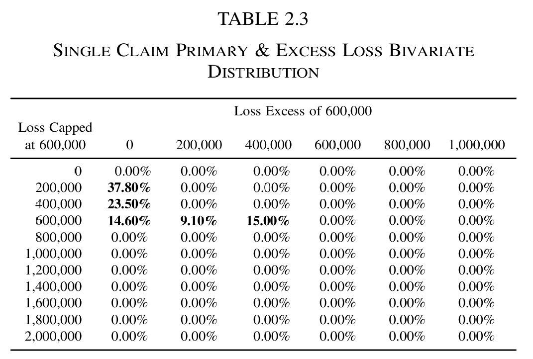
Section 2 is the sharpest of the three, because aggregate does not need Table 2.3 at all. The retained and ceded amounts are the net and ceded views of one occurrence layer, so the joint per-claim severity is the cession map pushed forward along the gross severity, and the object computes it. The paper spends a page constructing a matrix that is now a consequence of writing occurrence net of 400000 xs 600000.

The contrast with Jin et al. (2016), assessed on its own page, is worth drawing. That paper is dependence through a common shock on the claim counts, which aggregate cannot express. This one is dependence through a joint severity under a shared count, which is exactly what aggregate’s bivariate is. Jin and coauthors cite Clark and Homer for their FFT benchmark, so the two sit adjacent in the literature; they are on opposite sides of the feature boundary.

6.2 What the reproduction cost

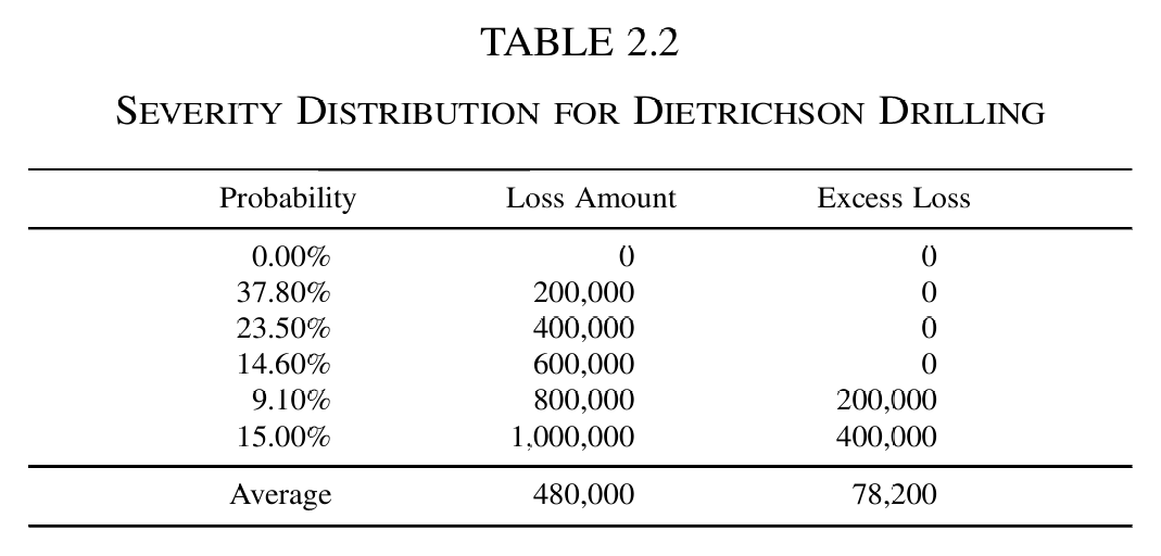
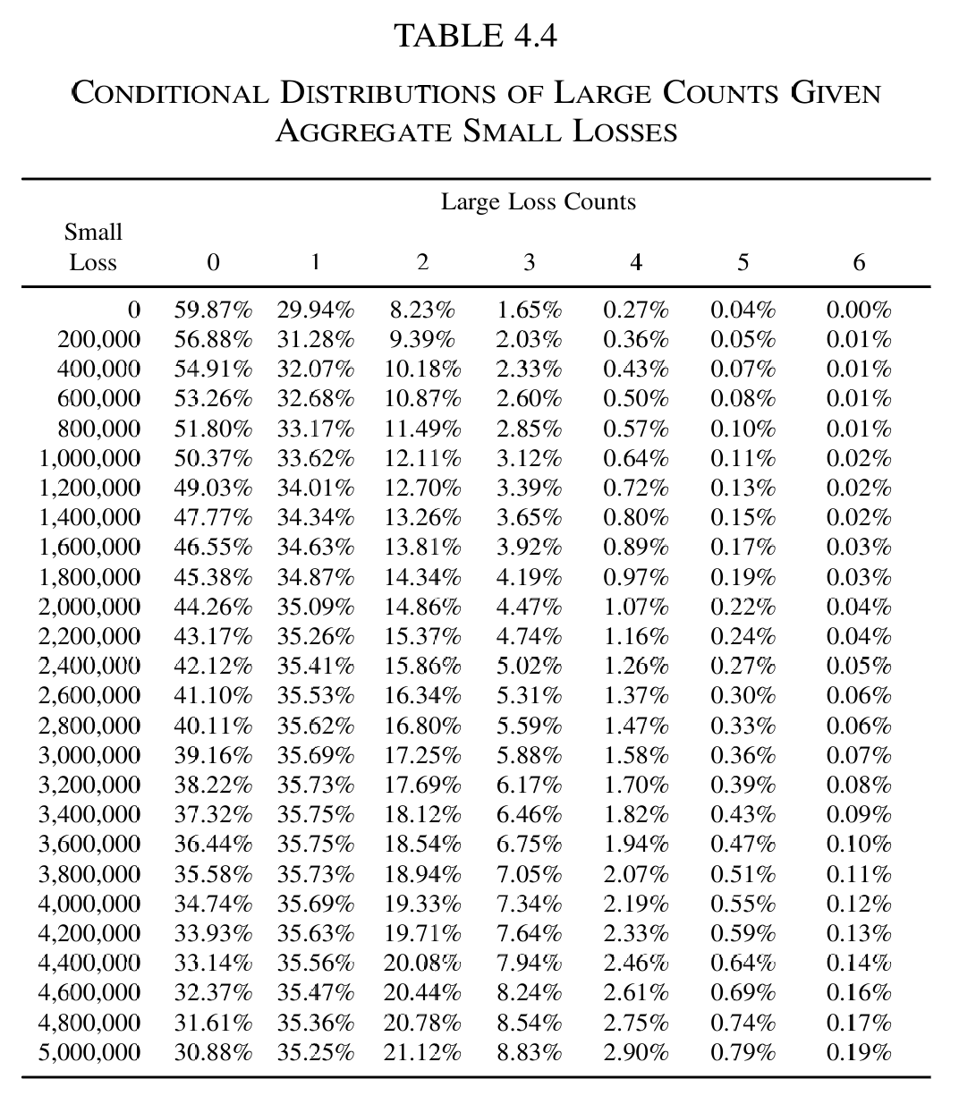
Table 19 scores every published block at once.

def score(got, paper):
    p = np.array(paper if isinstance(paper, np.ndarray) else list(paper.values()))
    return (got.size, int((np.round(got, 2) != np.round(p, 2)).sum()),
            float(np.abs(got - p).max()))

rows = []
for tag, got, pap in [('Appendix A, 3x3 convolution', None, None),
                      ('Section 2, Table 2.4', got24, pap24),
                      ('Section 3, Table 3.4', got34, T34),
                      ('Section 4, Table 4.3', got43, T43),
                      ('Section 4, Table 4.4', got44, T44)]:
    if got is None:
        rows.append({'target': tag, 'published cells': 9,
                     'cells differing at 2 dp': 0, 'worst raw difference': 0.0})
    else:
        n, diff, worst = score(got, pap)
        rows.append({'target': tag, 'published cells': n,
                     'cells differing at 2 dp': diff,
                     'worst raw difference': worst})
GT(pd.DataFrame(rows), float_format=4)

Table 19: Every published block, its cell count, how many differ at the two decimals printed, and the worst raw difference.

target	published cells	cells differing at 2 dp	worst raw difference
Appendix A, 3x3 convolution	9	0	0.0000
Section 2, Table 2.4	182	0	0.0050
Section 3, Table 3.4	147	11	0.0061
Section 4, Table 4.3	70	0	0.0050
Section 4, Table 4.4	28	0	0.0050

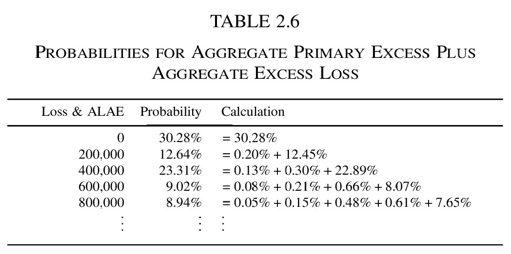
In Table 19, section 2 and section 4 reproduce every published cell at the two decimals printed, and the five section 2 statistics reproduce to the digit. Section 3 reproduces 136 of its 147 cells exactly and misses the other eleven by one unit in the last printed place.

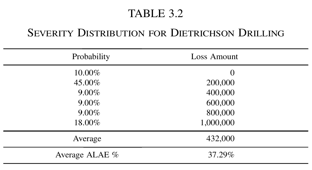
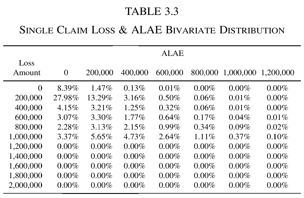
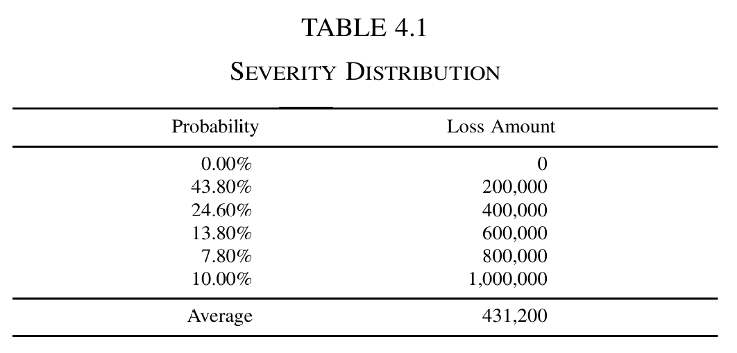
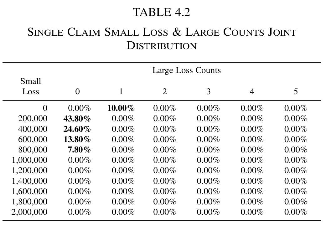
Those eleven are the price of the input matrix. Table 3.3 is itself printed to two decimals, so each of its 42 entries carries up to 0.005% of unstated error, and a four-fold convolution compounds that. Sections 2 and 4 do not have the problem because their inputs are exact: section 2’s severity matrix is derived from a five point severity by the cession map, and section 4’s is a five point severity with a single 10% atom. Where the paper gives an exact input, aggregate returns its exact output; where the paper gives a rounded input, the rounding survives.

6.3 Grid sizing is the one thing to get right

The first attempt at sections 3 and 4 used a \(2^6\) loss axis and returned garbage: two thirds of the mass missing in section 4 and nine tenths in section 3, and rows that looked like the paper’s but displaced several million dollars up the grid. The cause is that the pinned bucket size and log2 did not cover the measured window, so the window was clipped, and the object says so in Table 20.

small = build(dbvsev('HC4b', XS4, YS4, M4, 10, nb_cv(10, 20)),
              bs=(K, 1.0), log2=(6, 5))
GT(pd.DataFrame([
    {'log2 per axis': '(6, 5)', 'x reach': small.axis_xs[0][-1],
     'deficit': small.deficit},
    {'log2 per axis': '(7, 5)', 'x reach': gx4[-1], 'deficit': b4.deficit},
]))

V:\worktrees\aggregate_REFACTOR\src\aggregate\bivariate.py:1907: DefectiveDistributionWarning: bivariate HC4b: pinned (bs, log2) does not cover the measured window on an axis, so the joint loses mass off the grid -- raise log2, coarsen bs, or unpin one of them. Further occurrences this session are suppressed; each object records its own verdict in validation.
  bss, log2s, x_mins, his, clipped = self._size_axes(

Table 20: The section 4 build at two loss axis sizes, showing the reach and the mass deficit each gives.

log2 per axis	x reach	deficit
(6, 5)	16,600,000	678.958m
(7, 5)	25,400,000	529.132f

A deficit near 1, as in the first row of Table 20, is not a subtle warning, and it is the first thing to read off a bivariate build. Doubling one axis fixed it. This is the two-dimensional version of the padding discussion in the paper’s own Appendix C, where the error bound on the wrapped convolution is \(\|R\| \le \sum_{j>M} \mathsf P(N=j)\): run out of room and the mass does not disappear, it wraps.

6.4 Two blemishes in the paper

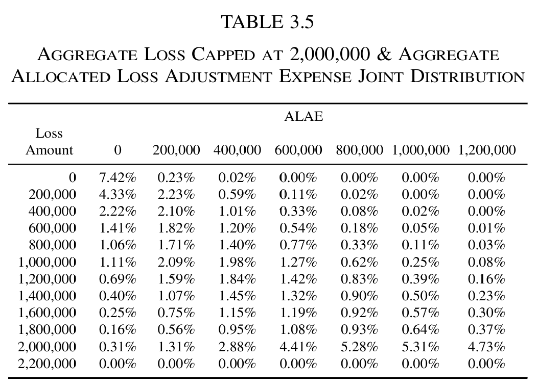
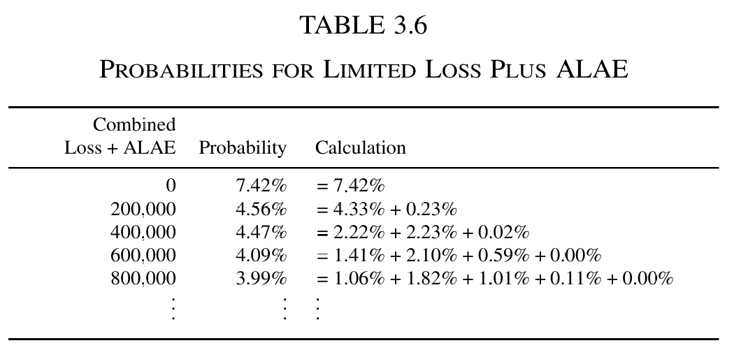
Table 3.3 does not sum to one. Printed to two decimals its rows give 10, 45, 9, 9, 9 and 17.97 percent against the 18 percent that Table 3.2 requires, so the matrix as published carries 99.97% of the mass. Scaling each row onto its Table 3.2 marginal is the correction, and with it Table 3.6 reproduces exactly; normalizing the whole matrix instead leaves Table 3.6 off by 0.01 in three of five cells.

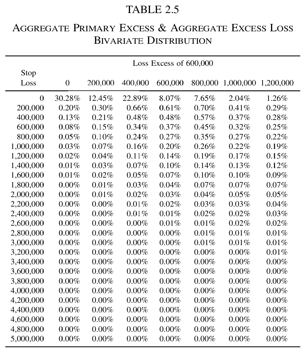
Table 2.6 is captioned “Loss & ALAE Probability Calculation” although it belongs to section 2 and concerns aggregate primary excess plus aggregate excess loss. The heading is a leftover from section 3.

Programs in the aggregate Loss Lab

Each program below opens in the aggregate Loss Lab, which builds it with nothing to install. The names are those in reproductions.agg, where every program is renamed by its paper’s citation key.

• Homer2003.A: the toy bivariate severity that checks the two dimensional convolution.
• Homer2003.HC: Section 2's per occurrence layer, whose net and ceded views give Table 2.3.
• Homer2003.HC3: Section 3's loss subject to an aggregate, plus unlimited ALAE.
• Homer2003.HC4: Section 4's joint distribution of dollars against counts.
• Homer2003.HC4b: Section 4's joint distribution on the smaller grid, for the reach comparison.

Homer, D. L., & Clark, D. R. (2003). Insurance Applications of Bivariate Distributions. Proceedings of the Casualty Actuarial Society, 90(iid), 274–307. http://www.casact.org/pubs/proceed/proceed03/03274.pdf

Jin, T., Provost, S. B., & Ren, J. (2016). Moment-based density approximations for aggregate losses. Scandinavian Actuarial Journal, 2016(3), 216–245. https://doi.org/10.1080/03461238.2014.921640

Mildenhall, S. J. (2005). Correlation and Aggregate Loss Distributions With An Emphasis On The Iman-Conover Method. Casualty Actuarial Society Forum, Winter. https://www.casact.org/sites/default/files/database/forum\_06wforum\_06w107.pdf