German liability insurers price increased limits by a rule Paul Riebesell published in 1936: doubling the sum insured multiplies the net premium by a constant factor \(1+z\), typically \(z = 20\%\). Written out,
a pure power law in the sum insured, and so invariant to inflation and to currency. That invariance is why it survives: unlike a property exposure curve it never needs re-basing.
Mack and Fackler (2003) asks whether the rule is consistent with the collective risk model, where \(b(v) = \mathsf E[N]\,\mathsf E[X \wedge v]\). Differentiating gives \(S(v) = b'(v)/\mathsf E[N]\), and a power law premium forces a power law survival function, that is a Pareto with
\[\alpha = 1 - \mathrm{ld}(1+z) \in (0,1).\]
An \(\alpha\) below one means an infinite mean, so the implied claim size law cannot be Pareto everywhere. The paper’s contribution is to show it does not have to be. There is a threshold \(u\) such that any realistic claim size law, fitted with a Pareto tail above \(u\), satisfies Riebesell’s rule exactly for all sums insured above \(u\), and the threshold turns out to sit below the range of sums insured actually written.
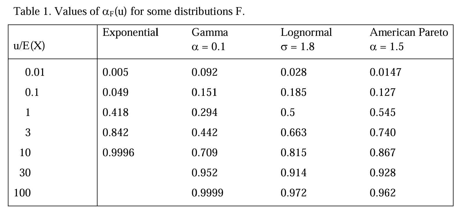
equals \(\alpha\). The quantity \(\alpha_F(u)\) runs from 0 at \(u=0\) to 1 as \(u \to \infty\) for any continuous \(F\) with a finite mean, so a solution always exists. Table 1, Figure 1, tabulates it for four severities at seven multiples of the mean, and it is the paper’s one block of numbers.
The formulation is convenient for aggregate: \(\alpha_F\) is built from a limited expected value and a survival function, both of which come straight out of a build.
Two readings had to be settled first. “American Pareto” is the two parameter Pareto \(S(x) = (\theta/(\theta+x))^\alpha\), lomax in DecL, as against the European single parameter form; with \(\alpha = 1.5\) the scale \(\theta = 0.5\) gives mean 1. “Gamma \(\alpha = 0.1\)” is the shape, so scale 10 for a unit mean. Both are confirmed by Table 1 reproducing.
3 The aggregate reproduction
Figure 1: Mack and Fackler (2003), Table 1.
def lev(prog, u, log2=20):"""E[X and u]: one fixed claim in the layer u xs 0."""return build(f'agg S 1 claim {u} xs 0 {prog} fixed', log2=log2, bs=u /2** (log2 -2), normalize=False).est_mdef sf(prog, u, log2=20):"""S(u) read off an unlimited build on a grid reaching well past u.""" obj = build(f'agg S 1 claim {prog} fixed', log2=log2, bs=4* u /2** log2, normalize=False)returnfloat(obj.density_df.loc[u, 'S'])rows = []for name, prog in SEVS.items():for i, u inenumerate(US): L, S = lev(prog, u), sf(prog, u) rows.append({'F': name, 'u / E(X)': u, 'agg E[X and u]': L,'agg S(u)': S, 'alpha_F(u)': 1- u * S / L,'Table 1': PAPER[name][i]})t1 = pd.DataFrame(rows)t1['abs diff'] = (t1['alpha_F(u)'] - t1['Table 1']).abs()GT(t1.set_index(['F', 'u / E(X)']), formatters={'agg E[X and u]': 6, 'agg S(u)': 6, 'alpha_F(u)': 6,'Table 1': 4, 'abs diff': '{x:.2e}'})
V:\worktrees\aggregate_REFACTOR\src\aggregate\_aggregate.py:4481: DefectiveDistributionWarning: S: aggregate PMF deficit 9.608e-01 (Σp = 1 − 9.608e-01 < 1); forwards and backwards S diverge by the deficit (forwards > backwards). Further occurrences this session are suppressed; each object records its own verdict in validation.
  rv = self.update_work(xs, debug=debug, x_min=x_min, x_max=x_max,
Table 1: \(\alpha_F(u)\) for the four severities at seven multiples of the mean, against Table 1.
Table 2: Worst cell error over the whole of Table 1.
cells compared
largest absolute difference
26
8.14e-04
By Table 2 all 26 cells land within \(8\times10^{-4}\), inside the paper’s three decimal rounding. The two blank cells are the exponential at \(u = 30\) and \(u = 100\), where \(\alpha_F\) is 1 to more places than the table prints and Mack and Fackler leave the entries empty.
Three exact statements in the text follow directly, in Table 3.
Table 3: The three constants the text quotes for \(z = 20%\), recomputed.
quantity
recomputed
paper
alpha = 1 - ld(1+z), z = 20%
0.736966
0.737000
exposure exponent 1 - alpha
0.263034
0.263000
mixed tail index alpha + beta, beta = 1.3
2.036966
2.037000
The last row of Table 3 is the paper’s resolution of an apparent contradiction. Riebesell forces \(\alpha < 1\) on the claim size law of a single risk, whereas observed portfolio tails in liability run near 2. Section 8 shows the two are compatible: mixing the individual laws over a Pareto distribution of sums insured with index \(\beta\) gives a portfolio tail of index \(\alpha + \beta\), and with \(\beta = 1.3\) that is 2.037.
4 Theorem 2, end to end
The theorem says: take any realistic \(F\), find the \(u\) solving \(\alpha_F(u) = \alpha\), replace the tail above \(u\) with a Pareto, and Riebesell’s rule holds exactly from \(u\) upward. The worked instance in the text is the lognormal with \(\sigma = 1.8\), for which the paper reads off Table 1 that “we replace the lognormal above \(u \approx 5 \cdot \mathsf E(X)\)”.
Scale to the paper’s own liability context, \(\mathsf E(X)\) below €50,000 and sums insured from about €500,000; Table 4 solves for the threshold.
import scipy.stats as ssfrom scipy.integrate import quadfrom scipy.optimize import brentqSIGMA, EX =1.8, 50_000.0LN_SCALE = EX * np.exp(-SIGMA **2/2)FZ = ss.lognorm(SIGMA, scale=LN_SCALE)U = brentq(lambda u: 1- u * FZ.sf(u) / quad(FZ.sf, 0, u, limit=300)[0] - ALPHA, EX, 20* EX, xtol=1e-6)SU =float(FZ.sf(U))GT(pd.DataFrame([{'E(X)': EX, 'threshold u*': U, 'u* / E(X)': U / EX,'paper': 'u ~ 5 E(X)', 'S(u*)': SU}]), formatters={'E(X)': '{x:,.0f}', 'threshold u*': '{x:,.1f}','u* / E(X)': 4, 'S(u*)': 8})
Table 4: The threshold \(u^*\) solving \(\alpha_F(u) = \alpha\) for the lognormal with \(\sigma = 1.8\), against the paper’s reading of Table 1.
E(X)
threshold u*
u* / E(X)
paper
S(u*)
50,000
259,286.7
5.1857
u ~ 5 E(X)
0.03480845
The splice is a DecL clause, so Theorem 2’s construction can be written rather than tabulated. Two components, each conditioned to its own interval: the lognormal below \(u^*\) and a single parameter Pareto with the Riebesell index above it, weighted \(1 - S(u^*)\) and \(S(u^*)\) so the survival function is continuous at the join.
Every limited expected value in Table 5 is read off one grid, which matters: a limited expected value computed on a grid tuned to its own limit is not comparable with one computed on a different grid when the severity has structure far below the limit, and this severity has all its density three orders of magnitude below the largest sum insured.
LOG2, BS =22, 5.0# x_max = 21.0M, covers every a belowdef lev_spliced(a):return build(f'agg Riebesell 1 claim {a:.10g} xs 0 {SPLICE} fixed', log2=LOG2, bs=BS, normalize=False).est_mv =5_000_000.0lev_v = lev_spliced(v)rows = []for a in [50_000., 100_000., 250_000., U, 500_000., 1e6, 2e6, 5e6]: ra = lev_spliced(a) / lev_v rows.append({'a': a, 'a >= u*': a >= U -1, 'agg E[X and a]': lev_spliced(a),'agg r(a)': ra, 'Riebesell (a/v)^0.263': (a / v) ** (1- ALPHA),'ratio': ra / (a / v) ** (1- ALPHA)})GT(pd.DataFrame(rows).set_index('a'), formatters={'agg E[X and a]': '{x:,.2f}', 'agg r(a)': 9,'Riebesell (a/v)^0.263': 9, 'ratio': 9})
Table 5: The loss elimination ratio off the spliced severity against Riebesell’s \((a/v)^{1-\alpha}\), above and below the threshold.
a
a >= u*
agg E[X and a]
agg r(a)
Riebesell (a/v)^0.263
ratio
50.000k
False
18,406.01
0.246296481
0.297804454
0.827040960
100.000k
False
25,103.44
0.335916800
0.357365344
0.939981466
250.000k
False
33,981.96
0.454723048
0.454762189
0.999913931
259.287k
True
34,312.44
0.459145281
0.459146069
0.999998283
500.000k
True
40,781.87
0.545714627
0.545714627
1.000000000
1.000M
True
48,938.24
0.654857552
0.654857552
1.000000000
2.000M
True
58,725.89
0.785829062
0.785829062
1.000000000
5.000M
True
74,731.12
1.000000000
1.000000000
1.000000000
In Table 5, above the threshold the loss elimination ratio matches Riebesell’s \((a/v)^{1-\alpha}\) to nine significant figures. Below it the agreement fails, and fails hard: at \(a = \mathsf E(X)\) the true ratio is 17% under the Riebesell value. That is not a numerical artifact, it is Theorem 2 being tight. The rule is not asymptotic or approximate above \(u\), and it is simply wrong below it.
The premium form of the same statement, Table 6, is sharper still, because the rule was stated as a premium rule in the first place.
GT(pd.DataFrame([{'sum insured v': v0, 'v >= u*': v0 >= U,'b(2v)/b(v) = E[X and 2v] / E[X and v]': lev_spliced(2* v0) / lev_spliced(v0),"Riebesell's 1 + z": 1.20}for v0 in [300_000., 600_000., 1_200_000., 100_000.]] ).set_index('sum insured v'), formatters={'b(2v)/b(v) = E[X and 2v] / E[X and v]': 6,"Riebesell's 1 + z": 2})
Table 6: The premium ratio on doubling the sum insured, at three sums insured above the threshold and one below.
sum insured v
v >= u*
b(2v)/b(v) = E[X and 2v] / E[X and v]
Riebesell's 1 + z
300,000
True
1.200000
1.20
600,000
True
1.200000
1.20
1,200,000
True
1.200000
1.20
100,000
False
1.270985
1.20
In Table 6, doubling the sum insured multiplies the collective risk premium by exactly 1.200000 at every sum insured above the threshold, and by 1.271 below it. A 1936 rating rule turns out to be an exact consequence of the collective risk model on the range where it is used, and only there.
5 Comments
5.1 What aggregate is doing here, and what it is not
This is a severity paper. There is no aggregate distribution anywhere in it: \(\mathsf E[N]\) enters every formula and cancels out of every one. aggregate is being used as a limited expected value engine on a spliced severity, which it does well, but the compound machinery is idle.
The reproduction is still worth having for two reasons. Mack and Fackler’s threshold condition is stated entirely in terms of \(\mathsf E[X \wedge u]\) and \(S(u)\), which are the two things exposure rating is built from, so the whole paper is one short expression away from quantities aggregate already reports. And Theorem 2’s construction is a splice clause: two components, two conditioning windows and two weights, which is the same shape as the theorem’s own statement. Mack2003.RiebesellPareto in the library carries the Riebesell index on its own, ground up rather than spliced, and has no finite mean, so it can only be used the way the paper uses it, inside a limit.
5.2 A grid caveat worth carrying forward
The first attempt at the exposure curve gave a clean power law with the wrong constant, off by 2.6%. The cause was giving each limit its own bucket size, bs = a / 2**17. That is normally sensible, but here the severity has essentially all its density below €300,000 while the largest limit is €5,000,000, so a grid tuned to the top limit puts the entire lognormal body in its first few buckets. Limited expected values that are going to be compared with each other have to come off a common grid. The version above uses one grid for all eight limits and the artifact disappears.
5.3 The far tail does not matter, and the paper says so
The Pareto tail with \(\alpha = 0.737\) has an infinite mean, so it has no unconditional moments to report. The splice clause carries it anyway, with no cutoff and no residual swept onto a last bin, because every limited expected value on this page is taken inside a limit, which is the only way the paper ever uses the curve. The paper says as much: “we can replace \(F_u\) above some very high amount \(w \gg u\) with something else, e.g. in order to ascertain a finite expectation”, because the behaviour of the law above the range where Riebesell is applied does not enter equation (2). Useful licence, and not needed here.
The construction is exact rather than approximate, which is why nine significant figures are available to agree to. The weights \(1 - S(u^*)\) and \(S(u^*)\) against the two conditioning windows reproduce \(S\) continuously at the join by definition, so the spliced survival function is the theorem’s \(F_u\), not a discretization of it.
One diagnostic follows from the missing moments and is worth naming so it is not read as an error. At some limits the Pareto component is capped to a point mass, its variance is zero to rounding and so comes out very slightly negative, and aggregate reports that along with a nan skewness. It reaches the moment diagnostics only. Limited expected values, which are all this page reads, are unaffected.
Programs in the aggregate Loss Lab
Each program below opens in the aggregate Loss Lab, which builds it with nothing to install. The names are those in reproductions.agg, where every program is renamed by its paper’s citation key.
Mack2003.S: a severity behind the Table 1 exposure curve, limited at one layer top.
Mack2003.S.v3: a severity behind the Table 1 exposure curve, unlimited.
Mack2003.S.v2: a severity behind the Table 1 exposure curve, limited at one layer top.
Mack2003.S.v4: a severity behind the Table 1 exposure curve, limited at one layer top.
Mack2003.S.v6: a severity behind the Table 1 exposure curve, unlimited.
Mack2003.S.v5: a severity behind the Table 1 exposure curve, limited at one layer top.
Mack2003.S.v7: a severity behind the Table 1 exposure curve, limited at one layer top.
Mack2003.S.v9: a severity behind the Table 1 exposure curve, unlimited.
Mack2003.S.v8: a severity behind the Table 1 exposure curve, limited at one layer top.
Mack2003.S.v10: a severity behind the Table 1 exposure curve, limited at one layer top.
Mack2003.S.v12: a severity behind the Table 1 exposure curve, unlimited.
Mack2003.S.v11: a severity behind the Table 1 exposure curve, limited at one layer top.
Mack2003.Riebesell: the spliced severity whose Pareto tail makes Riebesell's rule consistent.
Mack2003.Riebesell.v2: the spliced severity whose Pareto tail makes Riebesell's rule consistent.
Mack, T., & Fackler, M. (2003). Exposure-rating in liability reinsurance. Blätter der DGVFM, 26(2), 229–238.
5 Comments
5.1 What
aggregateis doing here, and what it is notThis is a severity paper. There is no aggregate distribution anywhere in it: \(\mathsf E[N]\) enters every formula and cancels out of every one.
aggregateis being used as a limited expected value engine on a spliced severity, which it does well, but the compound machinery is idle.The reproduction is still worth having for two reasons. Mack and Fackler’s threshold condition is stated entirely in terms of \(\mathsf E[X \wedge u]\) and \(S(u)\), which are the two things exposure rating is built from, so the whole paper is one short expression away from quantities
aggregatealready reports. And Theorem 2’s construction is aspliceclause: two components, two conditioning windows and two weights, which is the same shape as the theorem’s own statement.Mack2003.RiebesellParetoin the library carries the Riebesell index on its own, ground up rather than spliced, and has no finite mean, so it can only be used the way the paper uses it, inside a limit.5.2 A grid caveat worth carrying forward
The first attempt at the exposure curve gave a clean power law with the wrong constant, off by 2.6%. The cause was giving each limit its own bucket size,
bs = a / 2**17. That is normally sensible, but here the severity has essentially all its density below €300,000 while the largest limit is €5,000,000, so a grid tuned to the top limit puts the entire lognormal body in its first few buckets. Limited expected values that are going to be compared with each other have to come off a common grid. The version above uses one grid for all eight limits and the artifact disappears.5.3 The far tail does not matter, and the paper says so
The Pareto tail with \(\alpha = 0.737\) has an infinite mean, so it has no unconditional moments to report. The
spliceclause carries it anyway, with no cutoff and no residual swept onto a last bin, because every limited expected value on this page is taken inside a limit, which is the only way the paper ever uses the curve. The paper says as much: “we can replace \(F_u\) above some very high amount \(w \gg u\) with something else, e.g. in order to ascertain a finite expectation”, because the behaviour of the law above the range where Riebesell is applied does not enter equation (2). Useful licence, and not needed here.The construction is exact rather than approximate, which is why nine significant figures are available to agree to. The weights \(1 - S(u^*)\) and \(S(u^*)\) against the two conditioning windows reproduce \(S\) continuously at the join by definition, so the spliced survival function is the theorem’s \(F_u\), not a discretization of it.
One diagnostic follows from the missing moments and is worth naming so it is not read as an error. At some limits the Pareto component is capped to a point mass, its variance is zero to rounding and so comes out very slightly negative, and
aggregatereports that along with ananskewness. It reaches the moment diagnostics only. Limited expected values, which are all this page reads, are unaffected.