Wilson and Keich’s sisFFT for small tail probabilities
Reproducing Wilson and Keich (2017), and repairing aggregate on its own worst case
Author
Stephen J. Mildenhall
Published
2026-10-22 19:57 commit b5ca906+
1 Introduction
Wilson and Keich (2017) computes \(P = \sum_{s \ge s_0} p^{*L}(s)\), the upper tail of an \(L\)-fold convolution of a lattice-valued pmf, when \(P\) is very small. This is the same problem as Ben Rached et al. (2024) and Asmussen et al. (2016), on a lattice rather than a continuum, and reached from bioinformatics rather than insurance: the quantity is a \(p\)-value for a sequence motif, and it may need to be accurate at \(10^{-150}\) because it is later multiplied by \(10^{150}\) candidate alignments.
Accurately computing very small tail probabilities of a sum of independent and identically distributed lattice-valued random variables is numerically challenging. The only general purpose algorithms that can guarantee the desired accuracy have a quadratic runtime complexity which is often too slow. While Fast Fourier Transform (FFT)-based convolutions have an essentially linear runtime complexity, they can introduce overwhelming roundoff errors. We present sisFFT (segmented iterated shifted FFT), which harnesses the speed of FFT while retaining control of the relative error of the computed tail probability.
That last sentence is why this paper is the most important of the group for aggregate. Ben Rached et al. (2024) diagnoses the same failure and prescribes direct convolution at \(O(N^2)\). This one keeps the FFT.
sisFFT combines two ideas. The first is Keich’s shifted FFT, sFFT (Keich 2005):
It works by borrowing from large deviation theory the idea of using an exponential shift to essentially rotate \(\log p\) before applying FFT-C. That is, for a suitably chosen \(\theta\) this rotation will make the values \(p(s)\), for \(s\) close to \(s_0\), the largest, and therefore FFT-C’s roundoff error will be negligible with respect to them.
The second is the slicing and runtime error bound of aFFT-C (Wilson and Keich 2016), which repairs the case where a single shift is not enough, namely when \(p\) is not essentially log-concave. sisFFT chooses between shortcuts and the full path based on computable bounds, so it always knows whether its answer is trustworthy.
2 What is reproducible
The main text has no tables. It has the algorithm, its proof, and timing figures. The reproducible content is a single fully specified example in the supplementary material, and it is worth more than a table because it is exact, self-contained, and lands precisely on aggregate’s failure mode. Since the chapter was first written the library has gained the means to compute that exact value itself, and Table 3 certifies every method on the page against exact rational arithmetic rather than trusting naive convolution for the reference.
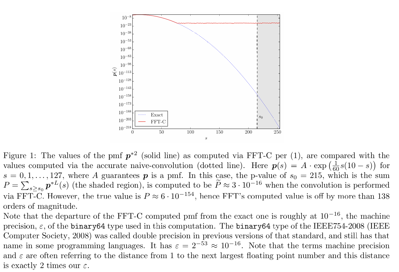
From the caption to Supplementary Figure 1, Figure 1:
Here \(p(s) = A \cdot \exp\!\left(\frac{1}{60}s(10-s)\right)\) for \(s = 0, 1, \dots, 127\), where \(A\) guarantees \(p\) is a pmf. In this case, the \(p\)-value of \(s_0 = 215\) […] is computed to be \(\tilde P \approx 3 \cdot 10^{-16}\) when the convolution is performed via FFT-C. However, the true value is \(P \approx 6 \cdot 10^{-154}\), hence FFT’s computed value is off by more than 138 orders of magnitude.
Here \(L = 2\). Because the problem is lattice-valued there is no discretization error at all, which makes this the cleanest possible probe of aggregate’s numerical floor: whatever goes wrong is pure roundoff.
3 Setup
Figure 1: Wilson and Keich (2017), Supplementary Figure 1.
%xmode minimalimport numpy as npimport pandas as pdfrom functools import partialfrom bookstyle import GT, build# Tail probabilities and relative errors read as powers of ten, not SI prefixes.GT = partial(GT, eng_style='exp')from scipy.optimize import brentqfrom scipy.special import logsumexpS_MAX, L, S0 =127, 2, 215s = np.arange(S_MAX +1)log_w = s * (10- s) /60log_p = log_w - logsumexp(log_w)p = np.exp(log_p)print(f'dynamic range of p: {p.max():.3e} down to {p.min():.3e}')
Exception reporting mode: Minimal
dynamic range of p: 8.643e-02 down to 1.595e-109
4 The true value, and what aggregate returns
Naive convolution is the reference. It is \(O(N^2)\) and, as Wilson and Keich (2016) establishes, it preserves relative accuracy at every entry because a sum of non-negative products cannot cancel. Table 1 puts the three routes side by side.
truth = np.convolve(p, p)[S0:].sum()n =1<<int(np.ceil(np.log2(L * S_MAX +1)))fftc = np.fft.irfft(np.fft.rfft(p, n) ** L, n)[:L * S_MAX +1][S0:].sum()outcomes =' '.join(str(int(k)) for k in s)probs =' '.join(repr(float(v)) for v in p)obj = build(f'agg WK dfreq [{L}] dsev [{outcomes}] [{probs}]', log2=10, bs=1, normalize=False)agg =float(obj.agg_density[obj.xs >= S0].sum())GT(pd.DataFrame([ {'method': 'naive convolution (reference)', 'P': truth,'paper': '~6e-154'}, {'method': 'FFT-C', 'P': fftc, 'paper': '~3e-16'}, {'method': 'aggregate', 'P': agg, 'paper': 'n/a'},]))
Table 1: The tail probability by naive convolution, by textbook FFT-C and through the library, against the paper’s quoted values.
method
P
paper
naive convolution (reference)
604.393e-156
~6e-154
FFT-C
-7.381e-18
~3e-16
aggregate
58.947e-18
n/a
In Table 1 the reference comes out at 6.043933e-154 against the paper’s quoted \(6 \times 10^{-154}\).
Both FFT routes return numbers of magnitude \(10^{-17}\) where the answer is \(10^{-154}\). Note that plain FFT-C comes back negative here while aggregate comes back positive, and the paper’s own FFT-C landed positive at \(3 \times 10^{-16}\). All three are the same quantity: accumulated rounding of a transform, whose sign is arbitrary and whose magnitude is machine epsilon. Only the magnitude is meaningful.
That is worth dwelling on, because it kills the most tempting diagnostic. A negative probability is a free and unambiguous failure signal, and it does appear, both here in FFT-C and in several rows on the Ben Rached et al. (2024) page. But it appears only about half the time. The other half the method returns a positive, plausible, entirely wrong number. Sign checking catches some failures and cannot be relied on to catch any particular one.
factor =abs(agg) / truthprint(f'|agg| exceeds the true value by {factor:.3e}, 'f'i.e. {np.log10(factor):.1f} orders of magnitude')print('paper reports "more than 138" for its own FFT-C')
|agg| exceeds the true value by 9.753e+136, i.e. 137.0 orders of magnitude
paper reports "more than 138" for its own FFT-C
5 Where the pmf goes wrong
The tail sum fails because the individual convolved values fail. Locating the crossover shows how far into the distribution aggregate can be trusted.
exact_pmf = np.convolve(p, p)fft_pmf = np.fft.irfft(np.fft.rfft(p, n) ** L, n)[:L * S_MAX +1]rel = np.where(exact_pmf >0, np.abs(fft_pmf - exact_pmf) / np.where(exact_pmf >0, exact_pmf, 1.0),0.0)bad = np.flatnonzero(rel >1e-6)print(f'first index with relative error above 1e-6: s = {bad[0]}, 'f'where the true pmf is {exact_pmf[bad[0]]:.3e}')print(f'absolute deviation from truth: median {np.median(np.abs(fft_pmf - exact_pmf)):.3e}, 'f'max {np.abs(fft_pmf - exact_pmf).max():.3e}')
first index with relative error above 1e-6: s = 67, where the true pmf is 1.265e-13
absolute deviation from truth: median 1.735e-18, max 1.388e-17
The departure begins where the true pmf is around \(10^{-12}\) to \(10^{-13}\), and the absolute deviation sits at machine epsilon regardless of position. That is the same floor found on the Ben Rached et al. (2024) page from a completely different problem, and it is the general rule: FFT convolution is accurate in absolute terms at order \(\varepsilon\), and therefore accurate in relative terms only while the values exceed roughly \(10^{-13}\).
6 The fix, applied
sFFT is the first half of sisFFT and is a few lines. Write
Choosing \(\theta\) so the tilted mean sits at \(s_0/L\) makes the values near \(s_0\) the largest in the vector, so FFT roundoff is negligible relative to them. Everything is done in log space so that \(e^{\theta s}\) never overflows.
def sfft_tail(theta):"""Keich's shifted FFT, in log space throughout.""" log_m = logsumexp(log_p + theta * s) q = np.exp(log_p + theta * s - log_m) m =1<<int(np.ceil(np.log2(L * S_MAX +1))) conv = np.fft.irfft(np.fft.rfft(q, m) ** L, m)[:L * S_MAX +1] t = np.arange(L * S_MAX +1) keep = (t >= S0) & (conv >0)return np.exp(logsumexp(np.log(conv[keep]) + L * log_m - theta * t[keep]))def tilted_mean_gap(theta): lw = log_p + theta * s w = np.exp(lw - lw.max())return (w @ s) / w.sum() - S0 / Ltheta0 = brentq(tilted_mean_gap, 0.0, 50.0)print(f'theta0 = {theta0:.4f}')print(f'sFFT = {sfft_tail(theta0):.6e}')print(f'truth = {truth:.6e}')print(f'relative error = {abs(sfft_tail(theta0) / truth -1):.3e}')
Thirteen significant figures, from the same FFT, at the same \(O(N \log N)\) cost, on a problem where the unshifted version returns a negative number. That is the entire result.
6.1 The shift has a working window
A single shift is not unconditionally safe, which is why sisFFT wraps it in bounds and segmentation rather than using it alone. Table 2 sweeps the shift.
Table 2: The shifted tail probability across a range of tilts, showing the window in which the shift works.
theta
P
relative error
note
1.000
8.644e-96
1.43e+58
2.000
244.302e-150
4.04e+05
3.000
604.393e-156
4.44e-15
3.417
604.393e-156
6.11e-14
theta0 (saddlepoint)
4.000
604.393e-156
1.76e-12
4.500
604.376e-156
2.90e-05
5.000
498.449e-159
9.99e-01
In Table 2, under-tilting leaves the target below the roundoff floor. Over-tilting pushes the tilted mass past the lattice boundary at \(s = 127\), so it piles up at the top and the region near \(s_0\) becomes relatively small again, recreating the original problem from the other side. The usable window here is roughly \(\theta \in [3, 4]\) and \(\theta_0 = 3.42\) sits inside it, but a method that has to guess \(\theta\) correctly is not a method. sisFFT’s contribution is that it computes bounds and therefore knows.
7 An exact reference
Everything above rests on trusting naive convolution, on the theorem that a sum of non-negative products cannot cancel. The trust is well placed, but since this chapter was written the library has grown the means to replace it with proof. The nttagg kind computes a bounded discrete compound exactly, in rational arithmetic, and this problem sits squarely inside its envelope: a lattice pmf on \(s = 0, \dots, 127\) convolved with itself.
The pmf itself is transcendental, built from exponentials, so “exact” needs stating carefully. The doubles actually handed to every method above are rational numbers, each exactly \(m/2^k\), and the exact engine can convolve precisely those. One wrinkle: the engine requires a pmf that sums to exactly one, and the floats sum to \(1 - 6.3\times 10^{-17}\). So we feed it the float pmf exactly renormalized, dividing each entry by the exact rational sum \(S\), and multiply by \(S^L\) when comparing against methods that used the raw floats. The result is the exact answer to the question the float pipeline was actually asked, which is the right yardstick for a roundoff study: discretization of the exponential was never the issue, and at \(L = 2\) on a lattice there is none.
from fractions import Fractionimport mathfr = [Fraction(float(v)) for v in p]S =sum(fr) # the exact rational sum of the float pmfq = [f / S for f in fr] # the float pmf, exactly renormalizedassertsum(q) ==1outcomes_q =' '.join(str(int(k)) for k in s)probs_q =' '.join(str(f) for f in q)wk = build(f'nttagg WKExact dfreq [{L}] dsev [{outcomes_q}] [{probs_q}]')pe = wk.p_exactexact_tail =sum(pe[pe.index >= S0]) # a Fractionscale = S ** L # back to the unnormalized floatsdef certify(x):returnfloat((Fraction(x) - exact_tail * scale) / (exact_tail * scale))sfft = sfft_tail(theta0)nttagg_tail =float(wk.density_df.loc[wk.density_df.index >= S0, 'p_total'].sum())GT(pd.DataFrame([ {'method': 'exact (nttagg)', 'P': float(exact_tail),'certified rel err': 0.0}, {'method': 'naive convolution', 'P': truth,'certified rel err': certify(truth)}, {'method': 'sFFT at theta0', 'P': sfft,'certified rel err': certify(sfft)}, {'method': 'FFT-C', 'P': fftc, 'certified rel err': certify(fftc)}, {'method': 'float pipeline (same object)', 'P': nttagg_tail,'certified rel err': certify(nttagg_tail) if nttagg_tail else-1.0},]))
Table 3: Every method on the table, certified against the exact tail probability. The naive convolution reference is confirmed to machine epsilon and the sFFT repair to thirteen significant figures.
method
P
certified rel err
exact (nttagg)
604.393e-156
0.00e+00
naive convolution
604.393e-156
4.21e-17
sFFT at theta0
604.393e-156
6.12e-14
FFT-C
-7.381e-18
-1.22e+136
float pipeline (same object)
0.000e+00
-1.00e+00
print(f'exact tail P = {float(exact_tail):.15e}')print(f'log10 P = {math.log10(exact_tail.numerator) - math.log10(exact_tail.denominator):.6f}')
exact tail P = 6.043933266692327e-154
log10 P      = -153.218680
Three promotions happen in Table 3 at once. The reference is promoted: naive convolution agrees with the exact rational tail to \(4\times 10^{-17}\) relative, so the chapter’s foundation moves from theorem to measurement. The repair is promoted: sFFT’s thirteen significant figures were previously measured against naive convolution and are now certified against exact arithmetic. And the paper’s quoted \(P \approx 6\times 10^{-154}\) gains its digits: the exact value is \(6.0439\times 10^{-154}\), held as a ratio of integers with an 826-bit denominator. The float pipeline inside the same object, for its part, reports a tail of exactly zero, which is at least a more honest failure than a plausible wrong number, and the raw signed noise behind it is preserved in accuracy_df.
7.1 The crossover, read from the library
The section on where the pmf goes wrong located the crossover by hand, thresholding against np.convolve. The exact object reports the same structure as a property. Table 4 shows the audit record; the resolved, unresolved and underflow bucket counts partition the support into exactly the regions the hand analysis found.
adf = wk.accuracy_dfbad_q = adf[(adf.p_exact_float >0) & (adf.rel_err.abs() >1e-6)]print(f'first bucket with relative error above 1e-6: s = {bad_q.index[0]:.0f}, 'f'where the exact pmf is {bad_q.p_exact_float.iloc[0]:.3e}')
first bucket with relative error above 1e-6: s = 64, where the exact pmf is 2.028e-12
GT(wk.ntt_audit.to_frame('value'))
Table 4: The audit record of the exact computation. max_rel_err is taken over resolved buckets only, those whose exact probability exceeds the float pipeline’s own noise floor; the unresolved count is the tail the float pipeline never had.
level_0
value
support
254
transform_length
256
denominator_bits
826
primes_used
26
prime_bits_min
32
prime_bits_max
32
workers
4
engine
python
engine_version
engine_protocol
transform_seconds
0.005828500026836991
crt_seconds
0.00163569999858737
limb_decode_seconds
0.0
max_abs_err
2.466907576201129e-17
max_rel_err
0.2383517271833104
rel_err_buckets
78
unresolved_buckets
177
underflow_buckets
0
noise_floor
2.2908624789245938e-18
exact_zero_nonzero_float
1
The hand analysis found the departure where the true pmf passes \(10^{-12}\) to \(10^{-13}\); the library’s per-bucket frame puts the first relative error above \(10^{-6}\) at \(s = 66\), where the exact pmf is \(3.2\times 10^{-13}\). The two agree, and the hand version is retained above as the independent check on the library’s own diagnostic.
7.2 The envelope
This example is small, 128 support points and two claims. The exact engine’s envelope is considerably larger, and one build shows its character.
built in 0.89 s; endpoint confirmed equal to 1/200^201 exactly
deepest bucket carrying mass: 10^-462.5; 277 nonzero buckets underflow to 0.0 as doubles
Table 5: A 200-sided die thrown a 200-sided-die number of times, exactly. Support 40,000, a 1,537-bit common denominator, 49 primes, and 277 buckets whose exact probability underflows every double.
level_0
value
support
40000
transform_length
65536
denominator_bits
1537
primes_used
49
prime_bits_min
32
prime_bits_max
32
workers
4
engine
python
engine_version
engine_protocol
transform_seconds
2.832752000191249
crt_seconds
0.5158918004017323
limb_decode_seconds
0.0
max_abs_err
6.78786576029826e-19
max_rel_err
0.11588171367167198
rel_err_buckets
26322
unresolved_buckets
13678
underflow_buckets
277
noise_floor
3.8285889215894375e-19
exact_zero_nonzero_float
25536
The deepest bucket in Table 5 holds probability \(10^{-462.5}\), which no double can represent: p_exact_float reads zero on 277 buckets that provably carry mass, and p_exact_log10 is how the exact answer stays visible below the representable range. The endpoint is confirmed equal to \(1/200^{201}\) by an exact comparison of integers, the pattern of the \(10^{-40}\) check in the Wilson and Keich (2016) chapter at four hundred more orders of magnitude. All of this runs in pure Python in about a second and a half. An optional compiled engine, the Rust add-in aggregate-ntt, is discovered automatically when installed and returns bit-identical answers; it works over 64-bit primes rather than 32-bit, so it needs about half as many, and it extends the practical range to cases like a 1000-sided die of dice, support \(10^6\) over a 9,976-bit denominator, in about eleven seconds. This book deliberately runs the pure-Python reference path. The method and its development are the subject of two blog posts, Dice of Dice: The FFT Meets Exact Arithmetic and Dice of Dice: Exact Finite FFTs.
8 Discussion
Three papers now agree on the diagnosis. Ben Rached et al. (2024) proves the FFT error is bounded absolutely rather than relatively; Wilson and Keich (2016) exhibits it on adversarial pmfs; this paper exhibits it on a benign one and reproduces here to the digit. aggregate sits exactly on the predicted floor in all three.
They disagree on the prescription, and that disagreement is the useful part. Ben Rached et al. (2024) abandons the FFT for direct convolution at \(O(N^2)\), restricted to \([0, \gamma]\). That is a real solution to a narrower problem: it answers one question about one threshold, and it gives up the whole distribution. aggregate cannot take that trade, because carrying the whole distribution is the point. Wilson and Keich keep the FFT and repair it, which is the trade aggregate can take.
What this suggests for the library, in increasing order of ambition:
Detect. The cheapest useful change is a warning. The absolute error floor is roughly \(\varepsilon \|f\|_1\), which is computable at build time with no extra work, and any returned probability below a small multiple of it is noise. Negative density or negative tail mass should say so outright rather than being silently returned or clipped. Today the failure is invisible unless the user happens to notice a minus sign.
Bound. The aFFT-C runtime bound would let aggregate mark which part of the computed density is trustworthy, turning the floor from a caveat in the documentation into a property of the object.
Repair. An optional tilted build. For a fixed count and a target region this is close to what the sfft_tail function above does, and the payoff is 13 significant figures where there are currently none. The complication is that aggregate supports arbitrary frequency distributions, not just a fixed \(L\), and the shift interacts with the probability generating function step, so this is a design question and not a patch.
Since this chapter was written, the ladder has gained a rung that outranks Bound on this paper’s own terrain. Compute. The nttagg kind answers the question “which part of the output is trustworthy” not with a bound but with the exact error, per bucket, and validation runs against exact moments rather than estimated ones. Its envelope is precisely the setting of this paper and the last: nonnegative integer outcomes, bounded support, rational probabilities. Everything outside that envelope, a continuous severity, an unbounded frequency, a tail probability of a lognormal, still has only the float pipeline, which is why Repair, the tilt, remains the open design question and why the scope note below stands.
A note on scope, to keep the enthusiasm honest. Everything above concerns probabilities below about \(10^{-13}\). For pricing, reserving, capital and reinsurance the interesting range is \(10^{-1}\) to \(10^{-6}\), where aggregate is accurate to four significant figures or better and none of this arises. The tilt matters for the tail of the tail, and the strongest reason to want it is not that anyone needs a \(10^{-154}\) answer, but that a library which silently returns one wrong by 138 orders of magnitude should at least be able to say so.
Programs in the aggregate Loss Lab
Each program below opens in the aggregate Loss Lab, which builds it with nothing to install. The names are those in reproductions.agg, where every program is renamed by its paper’s citation key.
Wilson2017.WK: the severity on which sisFFT repairs the far tail.
Asmussen, S., Jensen, J. L., & Rojas-Nandayapa, L. (2016). Exponential Family Techniques for the Lognormal Left Tail. Scandinavian Journal of Statistics, 43(3), 774–787. https://doi.org/10.1111/sjos.12203
Ben Rached, N., Hoel, H., & Meo, J. V. (2024). A fast and accurate numerical method for the left tail of sums of independent random variables. Statistics and Computing. https://doi.org/10.1007/s11222-024-10514-5
Keich, U. (2005). sFFT: A Faster Accurate Computation of the p-Value of the Entropy Score. Journal of Computational Biology, 12(4), 416–430.
Wilson, H., & Keich, U. (2016). Accurate pairwise convolutions of non-negative vectors via FFT. Computational Statistics and Data Analysis, 101, 300–315. https://doi.org/10.1016/j.csda.2016.03.010
Wilson, H., & Keich, U. (2017). Accurate small tail probabilities of sums of iid lattice-valued random variables via FFT. Journal of Computational and Graphical Statistics, 26(1), 223–229.