Mata and Verheyen on trend by layer

Reproducing Mata and Verheyen (2005)

Author

Stephen J. Mildenhall

Published

2026-10-22 19:56 commit b5ca906+

1 Context and problem

Two practical problems spoil excess of loss experience rating. Reinsurers often receive individual claim detail only above a reporting threshold, so lower layers cannot be trended claim by claim; and when the ceding company’s limits profile shifts during the experience period, averaging loss costs across years compares things that are not comparable.

Mata and Verheyen (2005) fixes both with the mathematics of exposure rating. A trend factor for a layer can be derived from the ground up trend, the severity curve and the limits profile, without touching individual claims, by asking what the expected severity in the layer costs at two claim cost levels:

\[(\text{Excess Trend})_p = \frac{\mathsf E_Y[Y \wedge T] - \mathsf E_Y[Y \wedge B]}{\mathsf E_X[X \wedge T] - \mathsf E_X[X \wedge B]},\]

with $T$ and $B$ the top and bottom of the layer capped at the policy limit. The same apparatus, run against two limits profiles instead of two cost levels, gives an exposure adjustment by layer. Both are then split into frequency and severity components, since the count of claims reaching a layer moves with ground up severity trend even when ground up frequency is flat.

Everything reduces to limited expected values, which makes it a clean aggregate exercise.

2 Paper solution and gold standard

The worked example runs through Tables 1 to 14, beginning with Figure 1. A ceding company writes limits from $250,000 to $5,000,000, severity is lognormal with $\mu = 9.31$ and $\sigma = 2.29$ in 2005 values, ground up severity trend is 8% a year, the expected gross loss ratio is 60%, and rates rose a cumulative 50% between 2000 and 2005. Five layers are priced. The 2000 severity is the same lognormal with $\mu' = \mu - \ln(1.08^5) = 8.93$.

The headline results are that the $4MM xs $1MM layer trends at 9.59% a year against an unlimited 8%, that the same layer’s exposure has doubled while total limits exposure rose only 9%, and that most of the excess trend is additional claims reaching the layer rather than larger claims within it.

%xmode minimal
import numpy as np
import pandas as pd
from bookstyle import GT, build

MU, SIGMA, TREND, YEARS, ELR, OL = 9.31, 2.29, 1.08, 5, 0.60, 1.50
CV = float(np.sqrt(np.exp(SIGMA ** 2) - 1))
M05 = float(np.exp(MU + SIGMA ** 2 / 2))
M00 = M05 / TREND ** YEARS
PL = [250e3, 500e3, 750e3, 1e6, 5e6]
SP05 = [2_250_000, 5_400_000, 2_925_000, 6_300_000, 9_000_000]
SP00 = [2_250_000, 4_500_000, 2_925_000, 3_150_000, 3_000_000]
LAYERS = [(250e3, 0.), (250e3, 250e3), (500e3, 500e3), (4e6, 1e6), (5e6, 0.)]
LN = ['$250k xs 0', '$250k xs $250k', '$500k xs $500k', '$4MM xs $1MM',
      '$5MM xs 0']
LOG2, BS = 20, 25.0                 # one grid, x_max = 26.2M

Exception reporting mode: Minimal

The 2000 mean uses the unrounded $\mu' = 8.925195$. Using the printed 8.93 instead moves the limited expected values by about half a percent, more than the effects the paper is measuring, and the paper’s own Table 1 is consistent with the unrounded value.

3 The `aggregate` reproduction

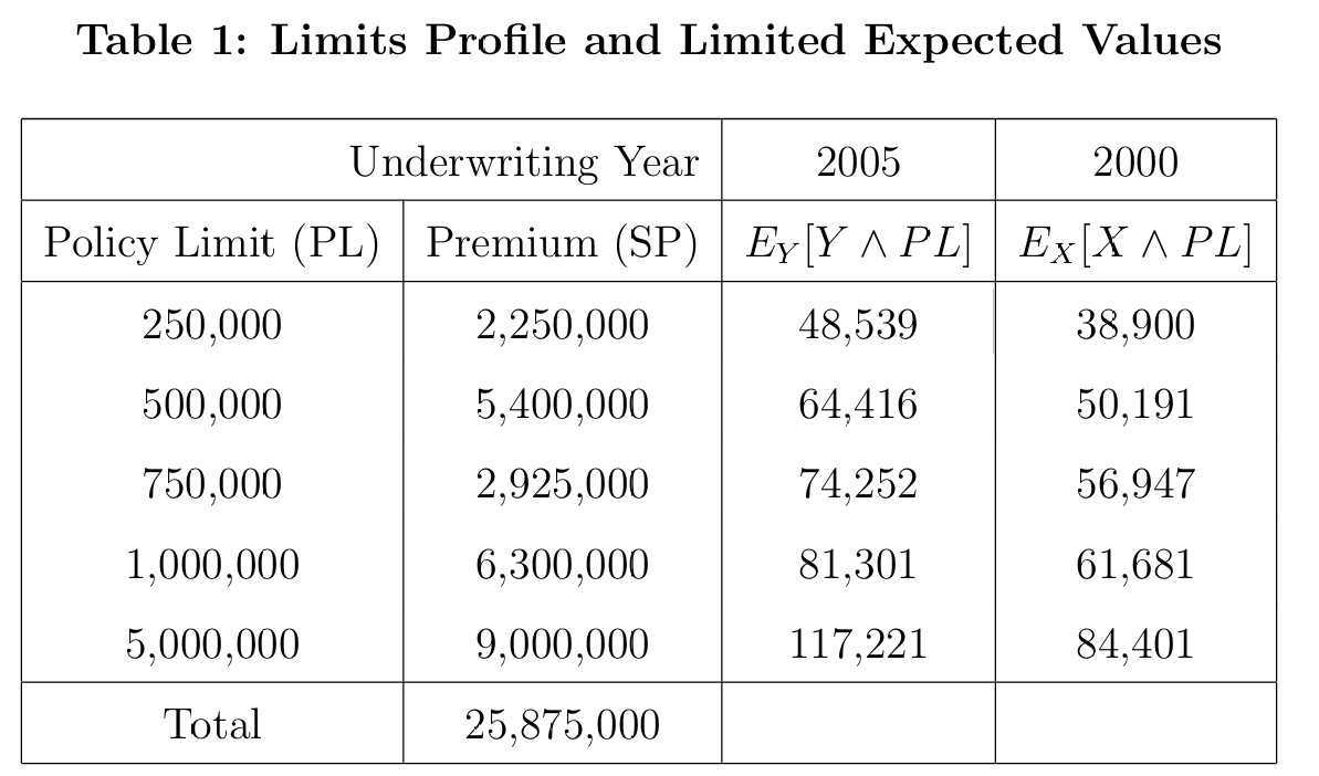
Figure 1: Mata and Verheyen (2005), Table 1.

def lev(a, mean):
    if a == 0:
        return 0.0
    return build(f'agg M 1 claim {a} xs 0 sev lognorm {mean} cv {CV} fixed',
                 log2=LOG2, bs=BS, normalize=False).est_m

PTS = sorted({0.} | set(PL) | {min(p, t + l) for p in PL for l, t in LAYERS}
             | {min(p, t) for p in PL for l, t in LAYERS})
AGG = {(a, y): lev(a, M05 if y == 2005 else M00)
       for y in (2005, 2000) for a in PTS}
PAP = {(p, 2005): v for p, v in zip(PL, [48539, 64416, 74252, 81301, 117221])}
PAP.update({(p, 2000): v for p, v in zip(PL, [38900, 50191, 56947, 61681, 84401])})
PAP.update({(0., 2005): 0.0, (0., 2000): 0.0})

t1 = pd.DataFrame({'policy limit': PL, 'premium 2005': SP05,
                   'agg EY[Y and PL]': [AGG[(p, 2005)] for p in PL],
                   'Table 1 2005': [PAP[(p, 2005)] for p in PL],
                   'agg EX[X and PL]': [AGG[(p, 2000)] for p in PL],
                   'Table 1 2000': [PAP[(p, 2000)] for p in PL]})
t1['2005 paper / agg'] = t1['Table 1 2005'] / t1['agg EY[Y and PL]']
t1['2000 paper / agg'] = t1['Table 1 2000'] / t1['agg EX[X and PL]']
GT(t1.set_index('policy limit'),
   formatters={'premium 2005': '{x:,.0f}', 'agg EY[Y and PL]': '{x:,.2f}',
               'Table 1 2005': '{x:,.0f}', 'agg EX[X and PL]': '{x:,.2f}',
               'Table 1 2000': '{x:,.0f}', '2005 paper / agg': 6,
               '2000 paper / agg': 6})

Table 1: Limited expected values at the five policy limits in both years, against Table 1.

policy limit	premium 2005	agg EY[Y and PL]	Table 1 2005	agg EX[X and PL]	Table 1 2000	2005 paper / agg	2000 paper / agg
250,000	2,250,000	48,519.84	48,539	38,895.61	38,900	1.000395	1.000113
500,000	5,400,000	64,424.73	64,416	50,214.86	50,191	0.999864	0.999525
750,000	2,925,000	74,289.42	74,252	56,996.34	56,947	0.999496	0.999134
1,000,000	6,300,000	81,363.94	81,301	61,752.27	61,681	0.999226	0.998846
5,000,000	9,000,000	117,503.76	117,221	84,637.21	84,401	0.997594	0.997209

In Table 1 the limited expected values do not agree. The paper is 0.04% high at $250,000 and drifts steadily to 0.24% low at $5,000,000, in both years. The discrepancy is small but it is systematic, and it is worth settling before reading anything downstream.

aggregate is not the source. The lognormal limited expected value has a closed form, $\mathsf E[X \wedge a] = e^{\mu + \sigma^2/2}\,\Phi\!\left(\frac{\ln a - \mu - \sigma^2}{\sigma}\right) + a\,S(a)$, and Table 2 arbitrates:

import scipy.stats as ss
FZ05 = ss.lognorm(SIGMA, scale=np.exp(MU))

def closed(a):
    return (M05 * ss.norm.cdf((np.log(a) - MU - SIGMA ** 2) / SIGMA)
            + a * FZ05.sf(a))

chk = pd.DataFrame({'a': PL, 'aggregate': [AGG[(p, 2005)] for p in PL],
                    'closed form': [closed(p) for p in PL],
                    'Table 1': [PAP[(p, 2005)] for p in PL]})
chk['agg / closed form - 1'] = chk['aggregate'] / chk['closed form'] - 1
chk['Table 1 / closed form - 1'] = chk['Table 1'] / chk['closed form'] - 1
GT(chk.set_index('a'),
   formatters={'aggregate': '{x:,.4f}', 'closed form': '{x:,.4f}',
               'Table 1': '{x:,.0f}', 'agg / closed form - 1': '{x:.2e}',
               'Table 1 / closed form - 1': '{x:.2e}'})

Table 2: The build and Table 1 each measured against the closed form lognormal limited expected value.

a	aggregate	closed form	Table 1	agg / closed form - 1	Table 1 / closed form - 1
250,000	48,519.8355	48,519.8377	48,539	-4.54e-08	3.95e-04
500,000	64,424.7341	64,424.7363	64,416	-3.42e-08	-1.36e-04
750,000	74,289.4170	74,289.4192	74,252	-2.97e-08	-5.04e-04
1,000,000	81,363.9371	81,363.9393	81,301	-2.71e-08	-7.74e-04
5,000,000	117,503.7600	117,503.7622	117,221	-1.88e-08	-2.41e-03

In Table 2, aggregate reproduces the closed form to better than five parts in a hundred million at every limit. Table 1 is out by up to twenty-four parts in ten thousand.

4 The decisive test

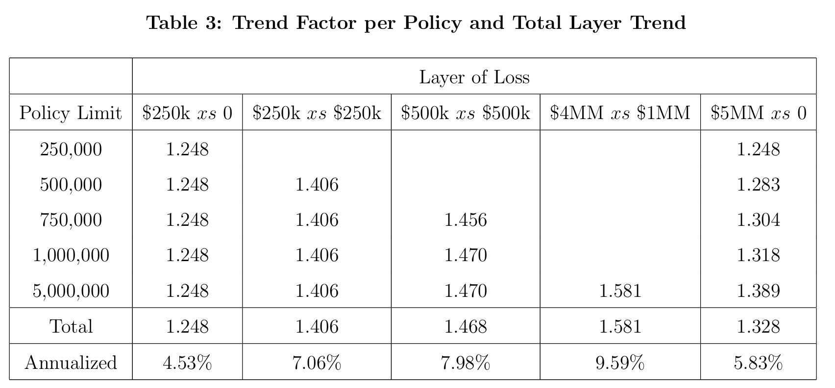
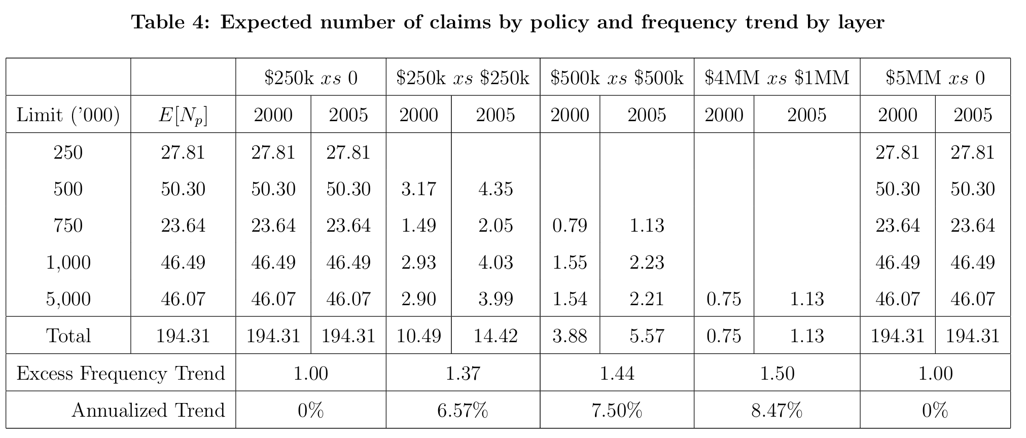
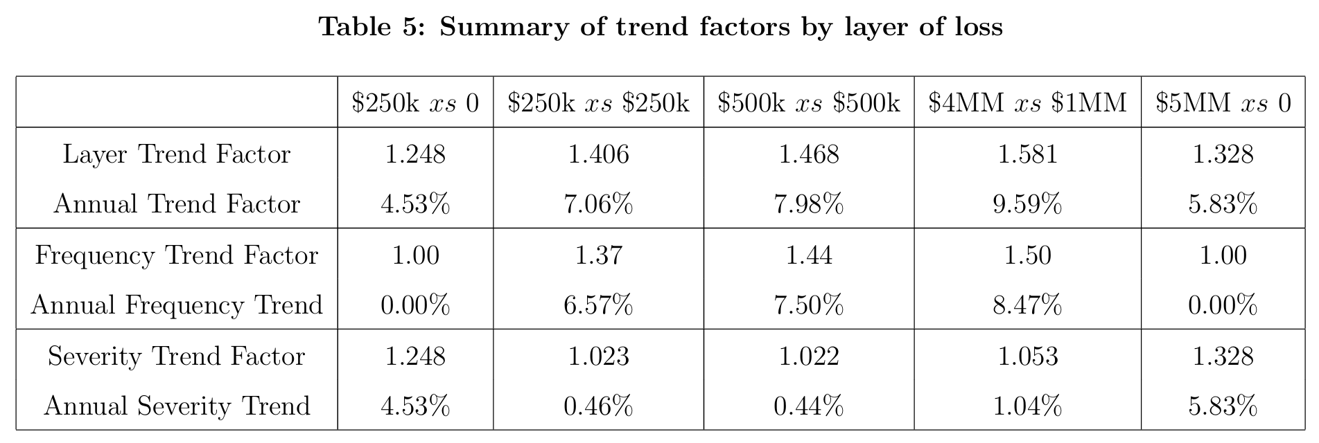
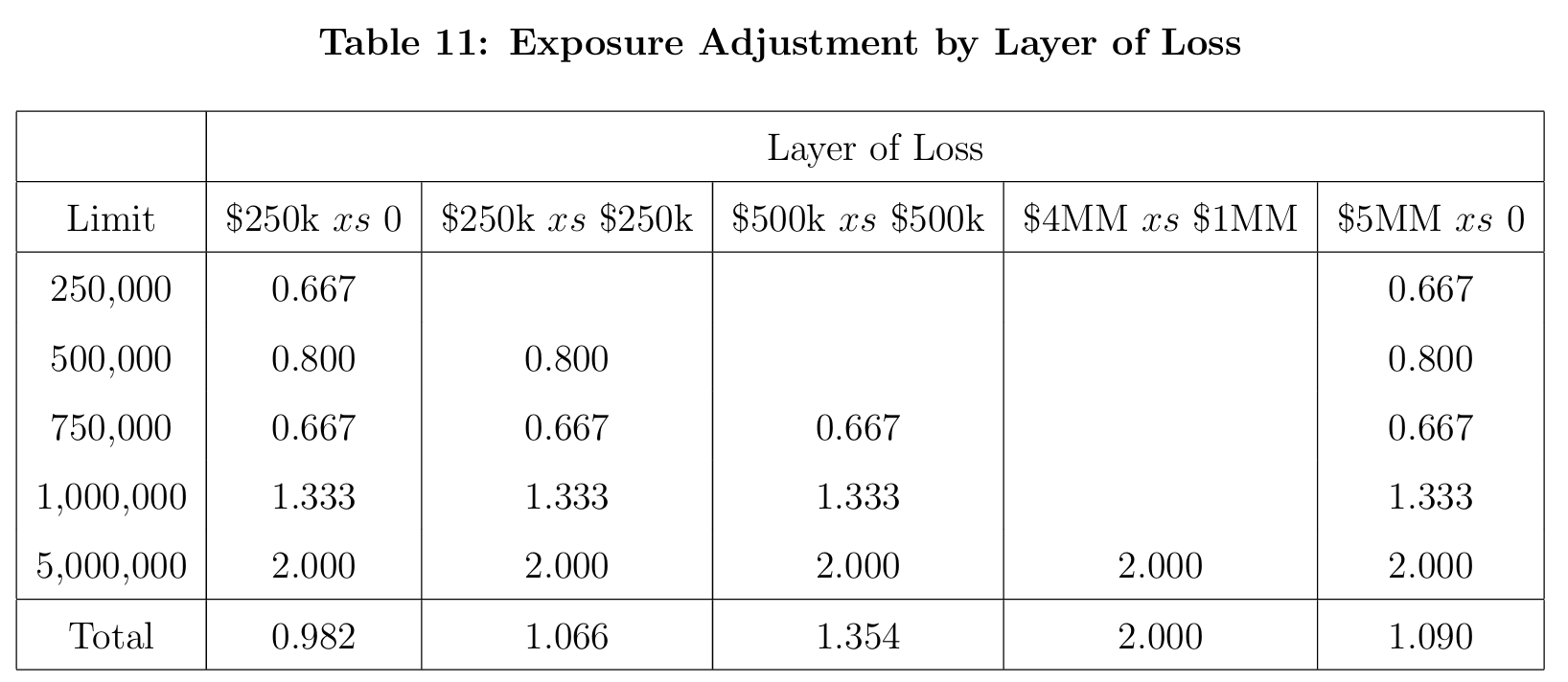
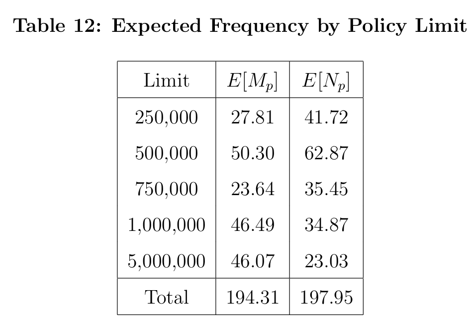
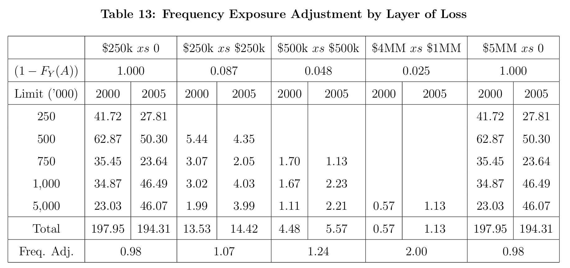
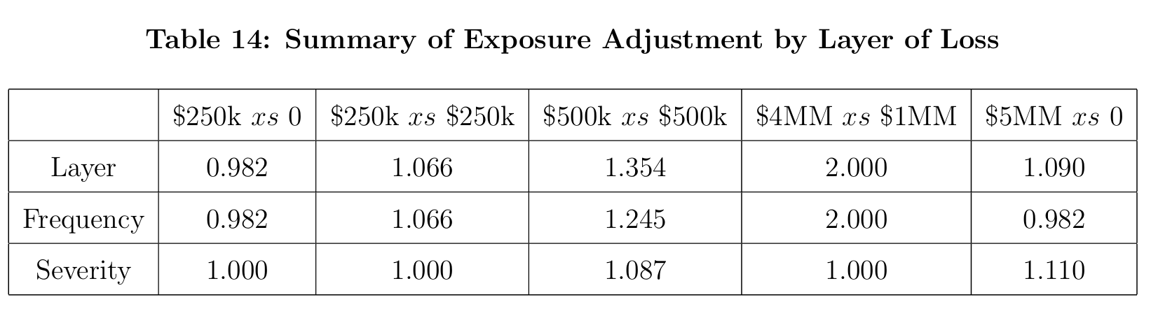
The question that matters is whether the method reproduces, so run the entire pipeline twice: once on aggregate’s limited expected values, once on the paper’s own Table 1 figures. The five policy limits happen to include every layer boundary the example needs, so the second run is possible with nothing but what the paper prints. The six published targets are Figure 2, Figure 3 and Figure 4 for the trend split, and Figure 5, Figure 7 and Figure 8 for the exposure split; Figure 6 carries the limits profiles both runs use.

Figure 2: Mata and Verheyen (2005), Table 3.

Figure 3: Mata and Verheyen (2005), Table 4.

Figure 4: Mata and Verheyen (2005), Table 5.

Figure 5: Mata and Verheyen (2005), Table 11.

Figure 6: Mata and Verheyen (2005), Table 12.

Figure 7: Mata and Verheyen (2005), Table 13.

Figure 8: Mata and Verheyen (2005), Table 14.

def sf(a, mean):
    if a == 0:
        return 1.0          # continuous severity, no atom at the origin
    return float(build(f'agg M 1 claim sev lognorm {mean} cv {CV} fixed',
                       log2=LOG2, bs=BS, normalize=False).density_df.loc[a, 'S'])

def pipeline(L):
    def lsev(p, limit, att, y):
        return L[(min(p, att + limit), y)] - L[(min(p, att), y)]

    pct = pd.DataFrame({n: [lsev(p, l, a, 2005) / L[(p, 2005)] for p in PL]
                        for n, (l, a) in zip(LN, LAYERS)},
                       index=[f'{p:,.0f}' for p in PL])
    lc05 = pct.mul(np.array(SP05) * ELR, axis=0)
    lc00 = pct.mul(np.array(SP00) * OL * ELR, axis=0)
    tr = pd.DataFrame({n: [(lambda d: lsev(p, l, a, 2005) / d if d > 0 else np.nan)
                           (lsev(p, l, a, 2000)) for p in PL]
                       for n, (l, a) in zip(LN, LAYERS)},
                      index=[f'{p:,.0f}' for p in PL])
    layer_trend = pd.Series({c: (tr[c] * lc05[c]).sum() / lc05[c].sum()
                             for c in tr.columns})
    EN = {p: s * ELR / L[(p, 2005)] for p, s in zip(PL, SP05)}
    EM = {p: s * OL * ELR / L[(p, 2005)] for p, s in zip(PL, SP00)}
    ft = {n: (sum(EN[p] * sf(a, M05) for p in PL if p > a)
              / sum(EN[p] * sf(a, M00) for p in PL if p > a))
          for n, (l, a) in zip(LN, LAYERS)}
    fa = {n: (sum(EN[p] * sf(a, M05) for p in PL if p > a)
              / sum(EM[p] * sf(a, M05) for p in PL if p > a))
          for n, (l, a) in zip(LN, LAYERS)}
    ea = lc05.sum() / lc00.sum()
    return pd.DataFrame({'T3 layer trend': layer_trend,
                         'T4 freq trend': pd.Series(ft),
                         'T5 sev trend': layer_trend / pd.Series(ft),
                         'T11 exposure adj': ea,
                         'T13 freq adj': pd.Series(fa),
                         'T14 sev adj': ea / pd.Series(fa)}), lc05

from_agg, lc_agg = pipeline(AGG)
from_paper, lc_paper = pipeline(PAP)
PRINTED = pd.DataFrame(
    {'T3 layer trend': [1.248, 1.406, 1.468, 1.581, 1.328],
     'T4 freq trend': [1.00, 1.37, 1.44, 1.50, 1.00],
     'T5 sev trend': [1.248, 1.023, 1.022, 1.053, 1.328],
     'T11 exposure adj': [0.982, 1.066, 1.354, 2.000, 1.090],
     'T13 freq adj': [0.982, 1.066, 1.245, 2.000, 0.982],
     'T14 sev adj': [1.000, 1.000, 1.087, 1.000, 1.110]}, index=LN)
GT(from_paper.rename_axis('layer'), float_format=4)

V:\worktrees\aggregate_REFACTOR\src\aggregate\_bucket_window.py:1430: InfeasibleGridWarning: M: severity 'lognorm' cannot be reproduced on this grid. The body needs bs <= 565.546 (7.5e-06% of the mean is supplied below the first half bucket, and is placed at 0); the mean is not complete until the grid reaches 15,491,470,518, so matching it to 0.0001 needs log2 = 25, and log2 = 20 was used. A thick unlimited severity has this problem at any bucket size, because its mean is furnished far above its median and a finer bs only shortens the reach. Add an occurrence limit, or accept the reported moment errors. Further occurrences this session are suppressed; each object records its own verdict in validation.
  warn_infeasible_grid(agg)
V:\worktrees\aggregate_REFACTOR\src\aggregate\_aggregate.py:4481: DefectiveDistributionWarning: M: aggregate PMF deficit 3.446e-04 (Σp = 1 − 3.446e-04 < 1); forwards and backwards S diverge by the deficit (forwards > backwards). Further occurrences this session are suppressed; each object records its own verdict in validation.
  rv = self.update_work(xs, debug=debug, x_min=x_min, x_max=x_max,
V:\worktrees\aggregate_REFACTOR\src\aggregate\_bucket_window.py:1430: InfeasibleGridWarning: M: severity 'lognorm' cannot be reproduced on this grid. The body needs bs <= 384.901 (1.843e-05% of the mean is supplied below the first half bucket, and is placed at 0); the mean is not complete until the grid reaches 10,543,234,532, so matching it to 0.0001 needs log2 = 25, and log2 = 20 was used. A thick unlimited severity has this problem at any bucket size, because its mean is furnished far above its median and a finer bs only shortens the reach. Add an occurrence limit, or accept the reported moment errors. Further occurrences this session are suppressed; each object records its own verdict in validation.
  warn_infeasible_grid(agg)

Table 3: The whole pipeline, Tables 3, 4, 5, 11, 13 and 14, driven by the paper’s own Table 1 figures.

layer	T3 layer trend	T4 freq trend	T5 sev trend	T11 exposure adj	T13 freq adj	T14 sev adj
$250k xs 0	1.2478	1.0000	1.2478	0.9816	0.9816	1.0000
$250k xs $250k	1.4062	1.3745	1.0230	1.0657	1.0657	1.0000
$500k xs $500k	1.4678	1.4358	1.0222	1.3535	1.2446	1.0875
$4MM xs $1MM	1.5810	1.5015	1.0529	2.0000	2.0000	1.0000
$5MM xs 0	1.3277	1.0000	1.3277	1.0900	0.9816	1.1105

GT(pd.DataFrame({"largest deviation, driven by the paper's Table 1":
                     (from_paper - PRINTED).abs().max(),
                 'largest deviation, driven by aggregate':
                     (from_agg - PRINTED).abs().max(),
                 'decimals the paper prints': [3, 2, 3, 3, 3, 3]}).rename_axis('quantity'),
   formatters={"largest deviation, driven by the paper's Table 1": 6,
               'largest deviation, driven by aggregate': 6,
               'decimals the paper prints': 0})

Table 4: Largest deviation from the printed values under each of the two runs, beside the precision the paper prints.

quantity	largest deviation, driven by the paper's Table 1	largest deviation, driven by aggregate	decimals the paper prints
T3 layer trend	0.000251	0.001804	3
T4 freq trend	0.004529	0.004529	2
T5 sev trend	0.000251	0.001268	3
T11 exposure adj	0.000463	0.000769	3
T13 freq adj	0.000398	0.000723	3
T14 sev adj	0.000492	0.000844	3

Table 3 is the answer and Table 4 scores it: driven by the paper’s own Table 1, every column reproduces to the last digit printed. The T4 freq trend column looks worse only because the paper prints it to two decimals, and it is identical in both runs since the frequency trend depends on survival probabilities alone and never touches a limited expected value.

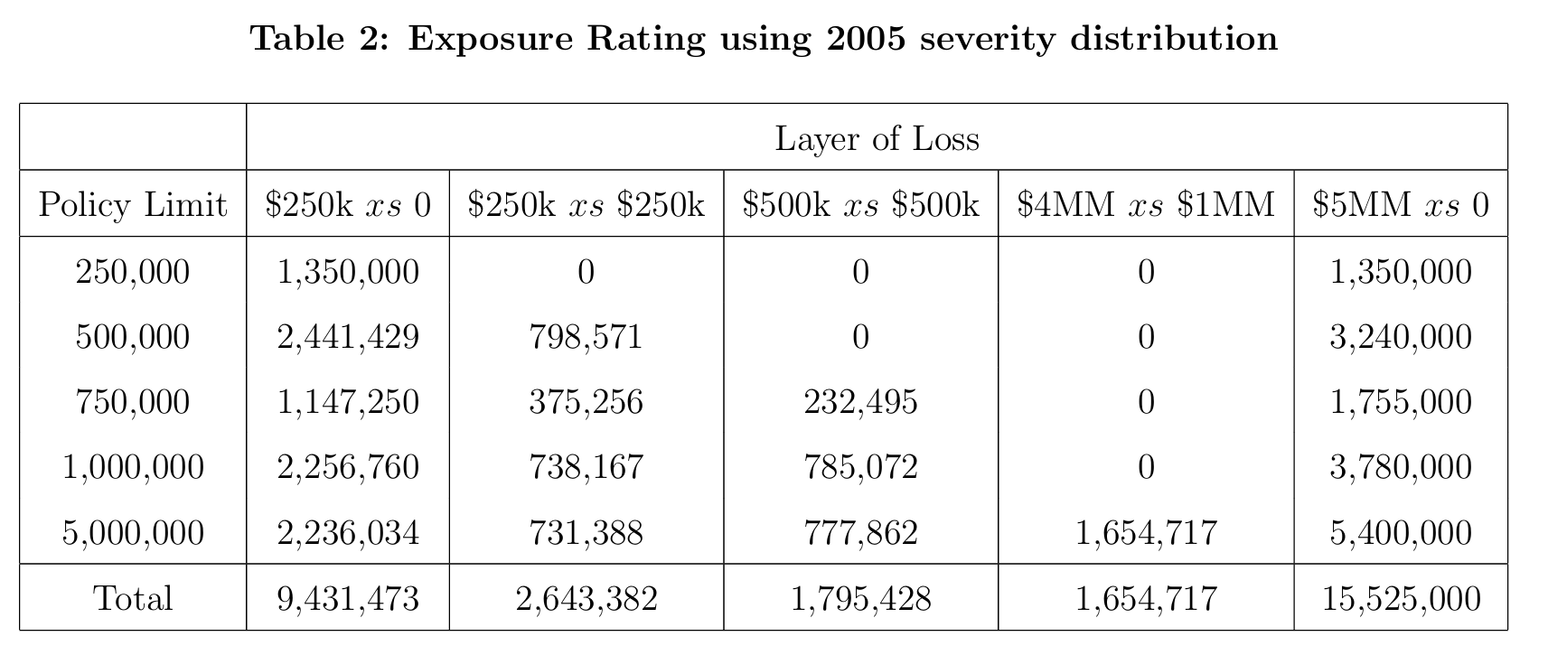
Table 2’s layer loss costs, Figure 9, come back within $60 on layers of up to $9.4 million in Table 5.

Figure 9: Mata and Verheyen (2005), Table 2.

GT(pd.DataFrame({'from paper Table 1': lc_paper.sum(),
                 'paper Table 2': [9_431_473, 2_643_382, 1_795_428, 1_654_717,
                                   15_525_000],
                 'from aggregate': lc_agg.sum()}).rename_axis('layer'), float_format=0)

Table 5: Layer loss costs from each run, against the printed Table 2.

layer	from paper Table 1	paper Table 2	from aggregate
$250k xs 0	9,431,477	9,431,473	9,420,254
$250k xs $250k	2,643,433	2,643,382	2,645,445
$500k xs $500k	1,795,369	1,795,428	1,798,459
$4MM xs $1MM	1,654,721	1,654,717	1,660,841
$5MM xs 0	15,525,000	15,525,000	15,525,000

So the implementation of the method is verified exactly, and the only discrepancy in the whole reproduction is Table 1. Driven by aggregate, the derived quantities move in the third decimal, as Table 6 sets out: the $4MM xs $1MM layer trend is 1.5792 rather than 1.5810, an annualized 9.57% rather than 9.59%.

GT(pd.DataFrame({'agg layer trend': from_agg['T3 layer trend'],
                 'agg annualized': from_agg['T3 layer trend'] ** (1 / YEARS) - 1,
                 'paper layer trend': PRINTED['T3 layer trend'],
                 'paper annualized': PRINTED['T3 layer trend'] ** (1 / YEARS) - 1,
                 'agg freq trend': from_agg['T4 freq trend'],
                 'agg freq annualized':
                     from_agg['T4 freq trend'] ** (1 / YEARS) - 1}).rename_axis('layer'),
   formatters={'agg layer trend': 4, 'paper layer trend': 4,
               'agg freq trend': 4, 'agg annualized': '{x:.2%}',
               'paper annualized': '{x:.2%}', 'agg freq annualized': '{x:.2%}'})

Table 6: Layer and frequency trend by layer, as multiples over five years and annualized, under both runs.

layer	agg layer trend	agg annualized	paper layer trend	paper annualized	agg freq trend	agg freq annualized
$250k xs 0	1.2474	4.52%	1.2480	4.53%	1.0000	0.00%
$250k xs $250k	1.4051	7.04%	1.4060	7.05%	1.3745	6.57%
$500k xs $500k	1.4664	7.96%	1.4680	7.98%	1.4358	7.50%
$4MM xs $1MM	1.5792	9.57%	1.5810	9.59%	1.5015	8.47%
$5MM xs 0	1.3273	5.83%	1.3280	5.84%	1.0000	0.00%

5 Comments

5.1 What is wrong with Table 1

The paper’s limited expected values are 0.04% high at the lowest limit and 0.24% low at the highest, in a smooth progression, in both years. That shape is the signature of a numerical integration that loses tail as the upper limit moves out, which is what a spreadsheet doing $\int_0^a x f(x)\,\mathrm dx$ on a fixed number of uniform steps would produce. A uniform-step trapezoid rule with roughly 900 to 1000 steps gets close to the pattern but does not match it at every limit, so the scheme is not identified here, only its symptom.

Nothing about the paper’s conclusions depends on it. The published deltas are large, a 9.59% layer trend against 8% unlimited, and a doubled exposure against a 9% total limits increase, and the third-decimal correction leaves all of them intact. The finding is worth recording because it is exactly the kind of thing a reproduction is for: two independent computations of the same quantity, one of which turns out to be a numerical approximation nobody flagged as one.

5.2 Reading the survival function of a very heavy lognormal

The frequency trend needs $S(A)$ at each attachment, and $\sigma = 2.29$ gives a coefficient of variation of 13.7. On a grid reaching $26M the build reports a mass deficit of $3.4\times10^{-4}$, which is severity mass above the grid, and the survival values carry a relative error of about $4\times10^{-5}$.

Pushing the grid out does not help, it hurts. Reaching far enough to make the deficit negligible would need $x_{\max} \approx 4\times10^{9}$, and at any affordable bucket count the discretization error then dominates: at bs = 3906 the survival error is $6\times10^{-3}$, two orders of magnitude worse than at bs = 25. For reading a survival function in the body of a distribution, resolution beats reach.

One related detail: the paper prints $1 - F_Y(A) = 1.000$ for the layers attaching at zero. A continuous severity has no atom at the origin, so the exact value is 1, but aggregate returns $F(0) = P(X \le \mathrm{bs}/2) = 0.0015$ at bs = 25. The code above returns 1 explicitly at $A = 0$ rather than reading it off the grid; without that the frequency trend for the two ground up layers comes out at 1.0011 instead of the correct 1.

5.3 Where the compound machinery would come in

As with Mack and Fackler (2003), this is a severity and layer paper. aggregate supplies limited expected values and survival probabilities; the frequency in equation (3.3) is a derived count, $\mathsf E[N_p] = (\mathrm{SP})(\mathrm{ELR})\beta_p / \mathsf E_Y[S_{Y,p}]$, not a distribution. The natural extension, which the paper does not take, is that once the layer expected loss and the claim count are both in hand, the layer’s aggregate distribution is one more DecL clause away, and with it the aggregate deductibles and reinstatements that a real treaty carries.

Programs in the aggregate Loss Lab

Each program below opens in the aggregate Loss Lab, which builds it with nothing to install. The names are those in reproductions.agg, where every program is renamed by its paper’s citation key.

Mata2005.M: the lognormal severity behind Table 1, limited at one layer top.
Mata2005.M.v2: the lognormal severity behind Table 1, limited at one layer top.
Mata2005.M.v3: the lognormal severity behind Table 1, unlimited.
Mata2005.M.v4: the lognormal severity behind Table 1, unlimited.

Mack, T., & Fackler, M. (2003). Exposure-rating in liability reinsurance. Blätter der DGVFM, 26(2), 229–238.

Mata, A. J., & Verheyen, M. A. (2005). An Improved Method for Experience Rating Excess of Loss Treaties using Exposure Rating Techniques. CAS Forum.