%xmode minimal
import numpy as np
import pandas as pd
from bookstyle import GT, build
Exception reporting mode: MinimalAssessing Jin, Provost and Ren (2016)
Jin et al. (2016) was ranked Tier 1 in the candidate assessment, on the reading that it offers “fully-specified Poisson/NegBin x Gamma/IG/Pareto with FFT comparison tables” and that one could “reproduce the FFT column exactly”. Reading the paper closely, that is not right, and the error is worth recording because it is easy to make from an abstract.
The paper has two halves. In the univariate half there are six fully specified compound models and no tabulated output at all: every result is a figure, and the numbered tables are Kolmogorov-Smirnov statistics computed against simulated samples, not distribution values. Exactly one published number in the whole half can be checked, and it checks out.
In the bivariate half there are eight tables with an FFT column, 96 reference values, and they are genuine. But the dependence structure is a common shock on the claim counts, which is not the dependence aggregate’s bivariate construct expresses. The joint law is reproducible with a short direct transform built on aggregate’s severity discretization, and it is reproduced below, but that is a demonstration of what the library would need rather than a use of what it has.
So: not a reproduction. What follows is the evidence.
The method is moment based. Approximate the density of \(S = X \mid X > 0\) by a gamma base density times a polynomial,
\[\tilde f_{S,t}(s) = g(s) \sum_{r=0}^{t} c_r s^r,\]
with \(g\) a gamma matched to the first two moments of \(S\) and the \(c_r\) recovered from a linear system matching the first \(t\). The appeal is that it needs only moments, so it works from sample moments when the frequency and severity are not separately known. The benchmark throughout is the FFT, which the authors treat as ground truth.
%xmode minimal
import numpy as np
import pandas as pd
from bookstyle import GT, buildException reporting mode: MinimalExample 1 is \(N \sim \mathrm{Poisson}(3)\), \(U \sim \gamma(3,2)\), polynomial order \(t = 15\). The text states: “it then follows from (2.4) that the base distribution is gamma (2.684349, 7.056877)”. Those two numbers are functions of the first two moments of \(S = X \mid X > 0\), with \(\tau = 1 - \mathsf P(N = 0)\) and \(\mu_S(a) = \mu_X(a)/\tau\), and Table 1 recovers them.
a = build('agg J 3 claims sev 2 * gamma 3 poisson', log2=18, bs=1 / 64,
          normalize=False)
tau = 1 - np.exp(-3.0)
ex1 = a.actual_m
ex2 = a.actual_m ** 2 * (1 + a.actual_cv ** 2)
mu1, mu2 = ex1 / tau, ex2 / tau
GT(pd.DataFrame([
    {'quantity': 'E[X]', 'aggregate': ex1, 'exact': 18.0},
    {'quantity': 'E[X^2]', 'aggregate': ex2, 'exact': 468.0},
    {'quantity': 'base gamma shape alpha',
     'aggregate': mu1 ** 2 / (mu2 - mu1 ** 2), 'exact': 2.684349},
    {'quantity': 'base gamma scale theta',
     'aggregate': (mu2 - mu1 ** 2) / mu1, 'exact': 7.056877},
]).set_index('quantity'), float_format=6)| quantity | aggregate | exact |
|---|---|---|
| E[X] | 18.000000 | 18.000000 |
| E[X^2] | 468.000000 | 468.000000 |
| base gamma shape alpha | 2.684349 | 2.684349 |
| base gamma scale theta | 7.056877 | 7.056877 |
Both to six figures in Table 1. This also pins the parameter conventions for the rest of the paper: \(\gamma(3,2)\) is shape 3 and scale 2, so mean 6, since any other reading misses the base gamma.
Table 2 builds all six and records what each publishes.
EX = [('1', 'agg J 3 claims sev 2 * gamma 3 poisson', 15,
       'Figures 1, 2, 3; Table 1 is K-S on simulated samples'),
      ('2', 'agg J 15 claims sev 2 * invgauss 1.5 poisson', 13,
       'Figures 4, 5, 6; Table 2 is K-S'),
      ('3', 'agg J 50 claims sev 2 * gamma 3 mixed gamma 0.3162277660168379',
       10, 'Figures 7, 8, 9; Table 3 is K-S'),
      ('4', 'agg J 50 claims sev 2 * invgauss 1.5 mixed gamma 0.3162277660168379',
       10, 'Figures 10, 11, 12; Table 4 is K-S'),
      ('5', 'agg J 3 claims sev 100 * lomax 20 poisson', 15,
       'Figures 13, 14, 15; Table 5 is K-S'),
      ('6', 'agg J 6 claims sev 100 * lomax 20 mixed gamma 0.5773502691896257',
       16, 'Figures 16, 17, 18; Table 6 is K-S')]
rows = []
for name, prog, t, published in EX:
    o = build(prog, log2=20, bs=1 / 32, normalize=False)
    rows.append({'example': name, 'DecL': prog.replace('agg J ', ''),
                 'order t': t, 'agg mean': o.est_m, 'agg CV': o.est_cv,
                 'published values': published})
GT(pd.DataFrame(rows).set_index('example'),
formatters={'agg mean': 4, 'agg CV': 4, 'order t': 0})| example | DecL | order t | agg mean | agg CV | published values |
|---|---|---|---|---|---|
| 1 | 3 claims sev 2 * gamma 3 poisson | 15 | 18.0000 | 0.6667 | Figures 1, 2, 3; Table 1 is K-S on simulated samples |
| 2 | 15 claims sev 2 * invgauss 1.5 poisson | 13 | 45.0000 | 0.4082 | Figures 4, 5, 6; Table 2 is K-S |
| 3 | 50 claims sev 2 * gamma 3 mixed gamma 0.3162277660168379 | 10 | 300.0000 | 0.3559 | Figures 7, 8, 9; Table 3 is K-S |
| 4 | 50 claims sev 2 * invgauss 1.5 mixed gamma 0.3162277660168379 | 10 | 150.0000 | 0.3873 | Figures 10, 11, 12; Table 4 is K-S |
| 5 | 3 claims sev 100 * lomax 20 poisson | 15 | 15.7894 | 0.8389 | Figures 13, 14, 15; Table 5 is K-S |
| 6 | 6 claims sev 100 * lomax 20 mixed gamma 0.5773502691896257 | 16 | 31.5789 | 0.8278 | Figures 16, 17, 18; Table 6 is K-S |
Every model builds in one line, which is why the paper looked like a good target. The last column of Table 2 is the problem. Tables 1 to 6 are the same six rows of Kolmogorov-Smirnov statistics at \(n = 100, 500, 1000, 10000\) with their critical values, and the statistic is computed between a simulated empirical distribution and the approximation fitted to that sample’s own moments. Nothing in it is a property of the model, so nothing in it is reproducible: a different seed gives different numbers, and the paper does not report one.
The translations above are worth keeping regardless. \(\mathrm{IG}(\eta, \theta)\) in the paper’s parameterization is {theta} * invgauss {eta/theta}; \(\mathrm{Pareto}(\gamma, \delta)\) with density \(\gamma\delta^\gamma/(u+\delta)^{\gamma+1}\) is {delta} * lomax {gamma}; and \(\mathrm{NB}(r, \beta)\) is a gamma-mixed Poisson with mean \(r\beta\) and mixing CV \(1/\sqrt{r}\), since matching \(n + n^2 c^2 = r\beta(1+\beta)\) at \(n = r\beta\) gives \(c^2 = \beta/n = 1/r\). The mixing CV does not depend on \(\beta\), which Table 3 confirms.
r, beta = 10.0, 5.0
c = 1 / np.sqrt(r)
nb = build(f'agg NB {r * beta} claims dsev [1] mixed gamma {c}', log2=12, bs=1,
           normalize=False)
GT(pd.DataFrame([{'mixing CV': c, 'mean': nb.est_m, 'want r*beta': r * beta,
                  'variance': nb.est_sd ** 2, 'want r*beta*(1+beta)':
r * beta * (1 + beta)}]), float_format=6)| mixing CV | mean | want r*beta | variance | want r*beta*(1+beta) |
|---|---|---|---|---|
| 0.316228 | 50.000000 | 50 | 300.000000 | 300 |
aggregate’s dependenceThe eight bivariate examples use Hesselager’s common shock counts: \(N = N_0 + N_1\) and \(W = N_0 + N_2\) with \(N_0, N_1, N_2\) independent, and all severities \(U_i, V_j\) mutually independent. Dependence between \(X\) and \(Y\) comes entirely from the shared count \(N_0\).
aggregate’s bivariate construct has a different shape. It puts a shared outer frequency over both perils and couples the two per-claim severities with a copula. To ask it for Hesselager’s model, thin the total count: with \(\lambda = \lambda_0 + \lambda_1 + \lambda_2\) events, each event independently triggers peril \(X\) with probability \(p_X = (\lambda_0+\lambda_1)/\lambda\) and peril \(Y\) with \(p_Y = (\lambda_0+\lambda_2)/\lambda\), and the two triggers must co-occur with probability \(\lambda_0/\lambda\). Table 4 is where that breaks down.
L0, L1, L2 = 7.0, 8.0, 9.0
L = L0 + L1 + L2
pX, pY = (L0 + L1) / L, (L0 + L2) / L
GT(pd.DataFrame([
    {'coupling of the two triggers': 'required by Hesselager',
     'P(both perils trigger)': L0 / L},
    {'coupling of the two triggers': 'independence copula',
     'P(both perils trigger)': pX * pY},
    {'coupling of the two triggers': 'comonotone, Frechet upper bound',
     'P(both perils trigger)': min(pX, pY)},
    {'coupling of the two triggers': 'countermonotone, Frechet lower bound',
     'P(both perils trigger)': max(0.0, pX + pY - 1)},
]).set_index('coupling of the two triggers'), float_format=6)| coupling of the two triggers | P(both perils trigger) |
|---|---|
| required by Hesselager | 0.291667 |
| independence copula | 0.416667 |
| comonotone, Frechet upper bound | 0.625000 |
| countermonotone, Frechet lower bound | 0.291667 |
In Table 4 the required probability is exactly the Fréchet lower bound, since \(p_X + p_Y - 1 = \lambda_0/\lambda\) identically. So there is a unique copula that gets the triggers right, and it is the countermonotone one. But the same copula then forces the two severities to be countermonotone whenever both perils fire, and Hesselager needs them independent. One copula cannot be countermonotone on the triggers and independent on the severities, so the model is outside the construct. This is a structural mismatch, not a parameterization difficulty.
The model is a two dimensional transform with a joint probability generating function. Since \(\mathsf P_{N,W}(z_1, z_2) = \mathsf P_{N_0}(z_1 z_2)\,\mathsf P_{N_1}(z_1)\,\mathsf P_{N_2}(z_2)\), the joint characteristic function of \((X, Y)\) is that pgf evaluated at the two severity transforms. aggregate supplies the severity discretization; the rest is a dozen lines. The target is Figure 1 and the result Table 5.
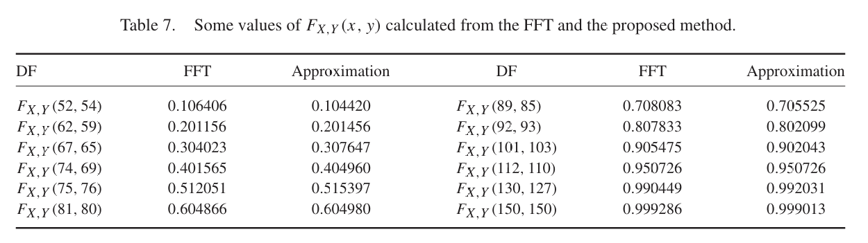
def joint(pgf, sev_u, sev_v, h, n):
    """Joint CDF of (X, Y) = (sum_{N0+N1} U, sum_{N0+N2} V) on an h-lattice."""
    du = build(f'agg U dfreq [1] {sev_u}', log2=int(np.log2(n)), bs=h,
               normalize=False).agg_density
    dv = build(f'agg V dfreq [1] {sev_v}', log2=int(np.log2(n)), bs=h,
               normalize=False).agg_density
    zu, zv = np.fft.fft(du), np.fft.fft(dv)
    g = np.fft.ifft2(pgf(zu[:, None], zv[None, :])).real
    return np.cumsum(np.cumsum(g, axis=0), axis=1)

H, N = 0.0625, 4096
F1 = joint(lambda z1, z2: np.exp(L0 * (z1 * z2 - 1) + L1 * (z1 - 1)
                                 + L2 * (z2 - 1)),
           'sev 2 * gamma 2', 'sev 1.5 * gamma 3', H, N)
T7 = [(52, 54, .106406), (62, 59, .201156), (67, 65, .304023),
      (74, 69, .401565), (75, 76, .512051), (81, 80, .604866),
      (89, 85, .708083), (92, 93, .807833), (101, 103, .905475),
      (112, 110, .950726), (130, 127, .990449), (150, 150, .999286)]
t7 = pd.DataFrame([{'x': x, 'y': y,
                    'direct 2-D transform': F1[int(round(x / H)), int(round(y / H))],
                    'Table 7 FFT': f} for x, y, f in T7])
t7['diff'] = (t7['direct 2-D transform'] - t7['Table 7 FFT']).abs()
GT(t7.set_index(['x', 'y']),
   formatters={'direct 2-D transform': 6, 'Table 7 FFT': 6,
'diff': '{x:.2e}'})| x | y | direct 2-D transform | Table 7 FFT | diff |
|---|---|---|---|---|
| 52 | 54 | 0.106478 | 0.106406 | 7.22e-05 |
| 62 | 59 | 0.201258 | 0.201156 | 1.02e-04 |
| 67 | 65 | 0.304145 | 0.304023 | 1.22e-04 |
| 74 | 69 | 0.401693 | 0.401565 | 1.28e-04 |
| 75 | 76 | 0.512181 | 0.512051 | 1.30e-04 |
| 81 | 80 | 0.604987 | 0.604866 | 1.21e-04 |
| 89 | 85 | 0.708186 | 0.708083 | 1.03e-04 |
| 92 | 93 | 0.807912 | 0.807833 | 7.91e-05 |
| 101 | 103 | 0.905521 | 0.905475 | 4.57e-05 |
| 112 | 110 | 0.950754 | 0.950726 | 2.79e-05 |
| 130 | 127 | 0.990455 | 0.990449 | 6.24e-06 |
| 150 | 150 | 0.999286 | 0.999286 | 4.75e-07 |
Bivariate Example 3 swaps Poisson for negative binomial counts, \(\mathrm{NB}(6,5)\), \(\mathrm{NB}(7,5)\), \(\mathrm{NB}(8,5)\), and needs only a different pgf. The target is Figure 2 and the result Table 6.
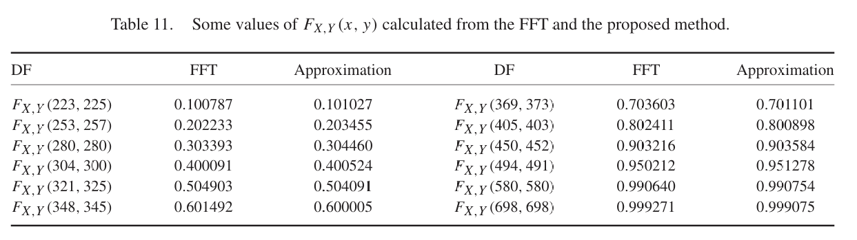
R0, R1, R2, BETA = 6.0, 7.0, 8.0, 5.0
def nb_pgf(z1, z2):
    P = lambda z, r: (1 - BETA * (z - 1)) ** -r
    return P(z1 * z2, R0) * P(z1, R1) * P(z2, R2)

H3 = 0.25
F3 = joint(nb_pgf, 'sev 2 * gamma 2', 'sev 1.5 * gamma 3', H3, 4096)
T11 = [(223, 225, .100787), (253, 257, .202233), (280, 280, .303393),
       (304, 300, .400091), (321, 325, .504903), (348, 345, .601492),
       (369, 373, .703603), (405, 403, .802411), (450, 452, .903216),
       (494, 491, .950212), (580, 580, .990640), (698, 698, .999271)]
t11 = pd.DataFrame([{'x': x, 'y': y,
                     'direct 2-D transform':
                         F3[int(round(x / H3)), int(round(y / H3))],
                     'Table 11 FFT': f} for x, y, f in T11])
t11['diff'] = (t11['direct 2-D transform'] - t11['Table 11 FFT']).abs()
GT(t11.set_index(['x', 'y']),
   formatters={'direct 2-D transform': 6, 'Table 11 FFT': 6,
'diff': '{x:.2e}'})| x | y | direct 2-D transform | Table 11 FFT | diff |
|---|---|---|---|---|
| 223 | 225 | 0.100985 | 0.100787 | 1.98e-04 |
| 253 | 257 | 0.202520 | 0.202233 | 2.87e-04 |
| 280 | 280 | 0.303725 | 0.303393 | 3.32e-04 |
| 304 | 300 | 0.400436 | 0.400091 | 3.45e-04 |
| 321 | 325 | 0.505241 | 0.504903 | 3.38e-04 |
| 348 | 345 | 0.601802 | 0.601492 | 3.10e-04 |
| 369 | 373 | 0.703865 | 0.703603 | 2.62e-04 |
| 405 | 403 | 0.802608 | 0.802411 | 1.97e-04 |
| 450 | 452 | 0.903326 | 0.903216 | 1.10e-04 |
| 494 | 491 | 0.950274 | 0.950212 | 6.18e-05 |
| 580 | 580 | 0.990653 | 0.990640 | 1.31e-05 |
| 698 | 698 | 0.999273 | 0.999271 | 1.71e-06 |
Table 5 and Table 6 both land within \(3.5\times10^{-4}\), with a residual that is uniformly positive, largest in the body of the distribution and vanishing in the tail. That is the signature of a half bucket offset rather than a disagreement about the model, and Table 7 confirms it by halving the bucket.
rows = []
for h, log2 in [(0.5, 9), (0.25, 10), (0.125, 11), (0.0625, 12)]:
    F = joint(lambda z1, z2: np.exp(L0 * (z1 * z2 - 1) + L1 * (z1 - 1)
                                    + L2 * (z2 - 1)),
              'sev 2 * gamma 2', 'sev 1.5 * gamma 3', h, 2 ** log2)
    rows.append({'bucket': h, 'grid': 2 ** log2, 'reach': h * 2 ** log2,
                 **{f'({x},{y})': F[int(round(x / h)), int(round(y / h))] - f
                    for x, y, f in [T7[0], T7[4], T7[8], T7[11]]}})
GT(pd.DataFrame(rows).set_index('bucket'),
   formatters={f'({x},{y})': '{x:.2e}'
for x, y, f in [T7[0], T7[4], T7[8], T7[11]]})| bucket | grid | reach | (52,54) | (75,76) | (101,103) | (150,150) |
|---|---|---|---|---|---|---|
| 0.50000 | 512 | 256 | 2.64e-03 | 4.60e-03 | 1.57e-03 | 1.69e-05 |
| 0.25000 | 1,024 | 256 | 1.16e-03 | 2.06e-03 | 7.20e-04 | 8.08e-06 |
| 0.12500 | 2,048 | 256 | 4.34e-04 | 7.77e-04 | 2.74e-04 | 3.11e-06 |
| 0.06250 | 4,096 | 256 | 7.22e-05 | 1.30e-04 | 4.57e-05 | 4.75e-07 |
In Table 7 the deviation falls monotonically at every halving, by a factor of thirty-five overall from bs = 0.5 to bs = 0.0625, so the paper’s FFT column is the exact joint distribution function and the reproduction agrees with it.
The candidate assessment suggested falling back on marginals. That does not rescue the reproduction, because the marginals miss precisely the quantity Figure 1 and Figure 2 are reporting, as Table 8 shows.
mx = build('agg X 15 claims sev 2 * gamma 2 poisson', log2=18, bs=1 / 32,
           normalize=False)
my = build('agg Y 16 claims sev 1.5 * gamma 3 poisson', log2=18, bs=1 / 32,
           normalize=False)
gap = pd.DataFrame([
    {'x': x, 'y': y, 'joint F(x,y)': F1[int(round(x / H)), int(round(y / H))],
     'FX(x) FY(y) under independence': (mx.density_df.loc[x, 'F']
                                        * my.density_df.loc[y, 'F']),
     'Table 7': f} for x, y, f in T7])
gap['dependence gap'] = gap['joint F(x,y)'] - gap['FX(x) FY(y) under independence']
GT(gap.set_index(['x', 'y']), float_format=6)| x | y | joint F(x,y) | FX(x) FY(y) under independence | Table 7 | dependence gap |
|---|---|---|---|---|---|
| 52 | 54 | 0.106478 | 0.071004 | 0.106406 | 0.035474 |
| 62 | 59 | 0.201258 | 0.158877 | 0.201156 | 0.042381 |
| 67 | 65 | 0.304145 | 0.259349 | 0.304023 | 0.044796 |
| 74 | 69 | 0.401693 | 0.363693 | 0.401565 | 0.038000 |
| 75 | 76 | 0.512181 | 0.474976 | 0.512051 | 0.037204 |
| 81 | 80 | 0.604987 | 0.577291 | 0.604866 | 0.027695 |
| 89 | 85 | 0.708186 | 0.691658 | 0.708083 | 0.016528 |
| 92 | 93 | 0.807912 | 0.796772 | 0.807833 | 0.011140 |
| 101 | 103 | 0.905521 | 0.901455 | 0.905475 | 0.004066 |
| 112 | 110 | 0.950754 | 0.949539 | 0.950726 | 0.001215 |
| 130 | 127 | 0.990455 | 0.990366 | 0.990449 | 0.000089 |
| 150 | 150 | 0.999286 | 0.999284 | 0.999286 | 0.000003 |
The margins are right: \(N = N_0 + N_1 \sim \mathrm{Poisson}(15)\) and \(W = N_0 + N_2 \sim \mathrm{Poisson}(16)\), both one-line builds. But the common shock moves the joint distribution function up to 4.5 points of probability away from the independent product, so a marginals-only reproduction would be reporting a number the paper never computed.
One feature: a common shock count mode for bivariate, in which the two components share a frequency component \(N_0\) and carry independent private components \(N_1\), \(N_2\), with severities independent throughout. That is the Hesselager model, it is standard in bivariate aggregate work, and the machinery to compute it is the twelve line joint function above sitting on the existing 2-D grid and severity discretization. It would turn 96 published reference values across eight tables into a regression suite, and it would give aggregate a count-driven dependence to sit beside the copula-driven one it already has.
Two smaller notes for whoever picks it up.
The paper has a specification defect in bivariate Example 6. The text reads “Let \(N_0 \sim \mathrm{NB}(5)\), \(N_1 \sim \mathrm{NB}(6)\), \(N_2 \sim \mathrm{NB}(7)\)”, giving one parameter to a two parameter family. The surrounding examples all use \(\beta = 5\), so \(\mathrm{NB}(5,5)\), \(\mathrm{NB}(6,5)\), \(\mathrm{NB}(7,5)\) is the obvious reading, but it is a guess and Tables 18 to 20 would decide it.
Tables 8, 10, 12, 14, 16, 17, 19, 20, 22 and 24 are simulation output and share the univariate half’s problem: they compare an empirical distribution from 5,000 simulated draws against the approximation fitted to that sample’s moments. Only the odd-numbered tables carry the FFT column that is worth anything as a reference.
Each program below opens in the aggregate Loss Lab, which builds it with nothing to install. The names are those in reproductions.agg, where every program is renamed by its paper’s citation key.
Jin2016.J: a test aggregate from the paper that did not reproduce.Jin2016.J.v2: a test aggregate from the paper that did not reproduce.Jin2016.J.v3: a test aggregate from the paper that did not reproduce.Jin2016.J.v4: a test aggregate from the paper that did not reproduce.Jin2016.J.v5: a test aggregate from the paper that did not reproduce.Jin2016.J.v6: a test aggregate from the paper that did not reproduce.Jin2016.NB: a negative binomial carrier, for the frequency check.Jin2016.U: a single claim severity from the bivariate convergence test.Jin2016.V: the other single claim severity from that test.Jin2016.X: a marginal of the paper's bivariate example.Jin2016.Y: the other marginal of that example.