Operational risk models push FFT convolution harder than insurance pricing does. The frequencies are moderate but the severities are extreme: a generalized Pareto with shape \(\xi = 1\) has no mean, let alone a variance, and the regulatory question is a high quantile of the aggregate. Schaller and Temnov (2008) is written from inside that problem, and its subject is how to get a trustworthy quantile out of an FFT when the severity has no moments to anchor the grid.
The paper compares three arrangements of the same transform. A naive FFT convolves on the grid as given, so aggregate mass that should land past the end wraps around into the low buckets. Padding by zeros extends the vector before transforming, so there is nowhere for the wrap to land. An exponential window multiplies the input by \(e^{-x/\tau}\) before transforming and divides it out afterwards, which is the exponential tilting of Grübel and Hermesmeier (1999) under another name, with the paper supplying a rule for the optimal \(\tau\).
The paper’s argument is that the exponential window matches the accuracy of generous padding at a fraction of the cost, and it makes that case with timings as well as accuracy.
2 Paper solution and gold standard
Section 4.3.2 is the real data example. The severity is a generalized Pareto in the form
with location \(\mu = 7000\), scale \(\beta = 12000\) and shape \(\xi = 1.0\). Frequency is Poisson with \(\lambda = 18\). The severity is truncated at \(x_m = 5\times 10^6\)and not normalized, which matters and is stated. The optimal window parameter is \(\tau_{\mathrm{opt}} = 149{,}688.5\).
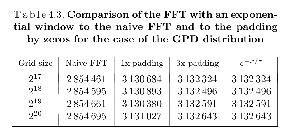
Table 4.3, Figure 1, then gives the 0.9-quantile of the aggregate at four grid sizes under all four arrangements. Its caption carries the detail that makes it reproducible: “The grid size indicated in the table is the one before the padding by zeros.” Table 1 transcribes it.
Table 1: Schaller and Temnov (2008), Table 4.3 as printed.
log2
naive
1x padding
3x padding
exponential window
17
2,854,461
3,130,684
3,132,324
3,132,324
18
2,854,595
3,130,893
3,132,496
3,132,496
19
2,854,661
3,130,380
3,132,591
3,132,591
20
2,854,695
3,131,027
3,132,643
3,132,643
Two features of Table 1 are worth naming before reproducing it. The naive column is wrong by 8.9%, which is the aliasing error and is far too large to be mistaken for anything subtle. And the exponential window column is identical to the 3x padding column at every grid size, to all seven digits. The paper’s own evidence is that the two remedies are interchangeable in accuracy, and its case for the window is therefore entirely about cost.
3 The aggregate reproduction
The severity is 12000 * genpareto 1 + 7000: scale, shape, location, in the order DecL takes them. aggregate’s padding counts doublings, so Schaller’s “1x padding” is padding=1 and his “3x padding”, a vector four times as long, is padding=2. The library has no exponential window on the production path, so that column has no counterpart here, which is the right outcome given the two are identical in the paper.
The grid is Schaller’s: the severity’s right endpoint is \(x_m = 5\times10^6\), so bs follows from the grid size rather than being chosen, for the reasons Table 2 records.
V:\worktrees\aggregate_REFACTOR\src\aggregate\_aggregate.py:4481: DefectiveDistributionWarning: SchallerTemnov: aggregate PMF deficit 5.568e-02 (Σp = 1 − 5.568e-02 < 1); forwards and backwards S diverge by the deficit (forwards > backwards). Further occurrences this session are suppressed; each object records its own verdict in validation.
  rv = self.update_work(xs, debug=debug, x_min=x_min, x_max=x_max,
GT(pd.DataFrame([ {'quantity': 'severity shape xi', 'value': 1.0,'note': 'xi = 1 means no finite mean'}, {'quantity': 'severity truncation x_m', 'value': XM,'note': 'stated in the paper, and not normalized'}, {'quantity': 'aggregate mass on the grid', 'value': a.agg_density.sum(),'note': 'below 1 by the truncated tail, as intended'},]).set_index('quantity'), formatters={'value': '{x:,.6g}'})
Table 2: The three features of the severity that make the grid an external choice rather than a computed one.
Table 4: Worst difference from Table 4.3, column by column and over all twelve values.
column
values compared
worst relative difference
worst absolute difference
naive
4
9.38e-05
268
1x padding
4
2.22e-04
695
3x padding
4
1.22e-04
382
all twelve
12
2.22e-04
695
By Table 3 and Table 4 all twelve distinct published values reproduce to within \(2.2\times10^{-4}\) relative, which on a quantile of 3.13 million is agreement to about 700. The aliasing error the paper is warning about, 8.9% of the answer, comes back at the same size; the two remedies both remove it; and the converged value is Schaller’s 3,132,643 to five significant figures.
3.1 Where the two calculations disagree, and it is instructive
The agreement is on the values. The pattern differs, and Table 5 shows it rather than averaging it away.
Table 5: The published and rebuilt columns side by side, showing the two implementations converging differently.
paper
aggregate
log2
naive
1x padding
3x padding
naive
1x padding
3x padding
17
2,854,461
3,130,684
3,132,324
2,854,729
3,131,065
3,132,706
18
2,854,595
3,130,893
3,132,496
2,854,729
3,131,065
3,132,687
19
2,854,661
3,130,380
3,132,591
2,854,729
3,131,075
3,132,687
20
2,854,695
3,131,027
3,132,643
2,854,729
3,131,075
3,132,687
In Table 5 Schaller’s columns rise monotonically with grid size: his 3x padding runs 3,132,324, 3,132,496, 3,132,591, 3,132,643, still climbing at \(2^{20}\). The aggregate column is flat from \(2^{18}\) onward at 3,132,687. Both land in the same place, but his estimate approaches it from below while this one is already there.
The reason is discretization, not aliasing. Refining the grid here refines bs as well, since \(x_m\) is fixed, so the sweep is a discretization sweep and the two implementations are converging at different rates from different discretization schemes. aggregate’s default preserves the cell mean, which is the moment-matching idea Gerber (1982) recommends; a scheme that assigns cell mass to an endpoint converges from one side, which is the shape of Schaller’s column. The residual 44 between 3,132,687 and 3,132,643 is about one bucket at \(2^{20}\), where bs is 4.77, so it is inside the quantile’s own quantization.
4 Comments
4.1 Normalization is not a cosmetic choice here
The paper says the severity is truncated and not normalized, and with \(\xi = 1\) that instruction is load bearing. Normalizing divides the truncated severity by its own mass, which redistributes the discarded tail proportionally across the retained buckets. For a thin tail that is a rounding correction. For a severity with no mean it is a change of model, and it thins the tail, as Table 6 measures.
Table 6: Two quantiles with and without normalization, at a coarse and a fine grid.
log2
normalize
0.9 quantile
0.99 quantile
mass on grid
17
False
3,132,706
4,999,962
0.94431685
True
2,456,551
4,999,962
0.98588811
20
False
3,132,687
4,999,995
0.94431707
True
2,456,560
4,999,995
0.98588820
In Table 6, normalizing moves the 0.9-quantile by a visible amount and the 0.99-quantile by more, always downward, because the mass removed from beyond the truncation point is being handed back to buckets below it. Anyone reproducing this table with normalize=True, which is aggregate’s default, will miss every entry and will miss it in a consistent direction. The general rule the library documents is the one this example forces: when the truncation error is unavoidable, do not normalize, and read the tail knowing it is understated.
4.2 The timing argument has not survived, and the accuracy argument never needed to
The paper’s case for the exponential window is cost: it reports the window giving the same precision as 2x padding in a third of the time, and as 3x padding at least four times faster. That was a real argument in 2008.
It is no longer the deciding one, because the whole sweep above, twelve builds up to \(2^{20}\) buckets with quadruple padding, runs in seconds. When the expensive option is cheap in absolute terms, a method that buys speed at the cost of a tuning parameter stops being attractive. And the window does carry one: \(\tau_{\mathrm{opt}} = 149{,}688.5\) is a computed quantity specific to this model, and getting it wrong costs accuracy in one direction or floating point range in the other, which is the failure mode Grübel and Hermesmeier (1999) hits at \(\theta N = 25\).
What Table 1 actually establishes, and states more strongly than the paper’s own argument needs, is that the window and generous padding are the same answer to seven digits at every grid size tested. Given that, the choice between them is entirely about which is easier to get right, and padding has no parameter to get wrong.
4.3 A severity with no mean is a good test of the grid sizer, and this one bypasses it
aggregate will refuse to pick a bucket size for an infinite-variance severity rather than guess, and \(\xi = 1\) has no mean at all. That refusal is why every build on this page carries an explicit bs in its hints{}, and why the sweep is expressed as \(x_m / 2^{\mathrm{log2}}\): the paper fixes the truncation point, so the grid size determines bs rather than the other way round.
That is the right way round for this problem and the wrong way round for most. Ordinarily bs is chosen from the severity’s own scale and the grid is made long enough to hold the aggregate. Here there is no scale to work from, so an external decision, the regulatory truncation point, supplies it.
Programs in the aggregate Loss Lab
Each program below opens in the aggregate Loss Lab, which builds it with nothing to install. The names are those in reproductions.agg, where every program is renamed by its paper’s citation key.
Gerber, H. U. (1982). On the numerical evaluation of the distribution of aggregate claims and its stop-loss premiums. Insurance Mathematics and Economics, 1(1), 13–18. https://doi.org/10.1016/0167-6687(82)90016-6
Grübel, R., & Hermesmeier, R. (1999). Computation of Compound Distributions I: Aliasing Errors and Exponential Tilting. Astin Bulletin, 29(2), 197–214. https://doi.org/10.2143/AST.29.2.504611
Schaller, P., & Temnov, G. (2008). Efficient and Precise Computation of Convolutions: Applying FFTs to Heavy Tailed Distributions. Computational Methods in Applied Mathematics, 8(2), 187–200.
4 Comments
4.1 Normalization is not a cosmetic choice here
The paper says the severity is truncated and not normalized, and with \(\xi = 1\) that instruction is load bearing. Normalizing divides the truncated severity by its own mass, which redistributes the discarded tail proportionally across the retained buckets. For a thin tail that is a rounding correction. For a severity with no mean it is a change of model, and it thins the tail, as Table 6 measures.
In Table 6, normalizing moves the 0.9-quantile by a visible amount and the 0.99-quantile by more, always downward, because the mass removed from beyond the truncation point is being handed back to buckets below it. Anyone reproducing this table with
normalize=True, which isaggregate’s default, will miss every entry and will miss it in a consistent direction. The general rule the library documents is the one this example forces: when the truncation error is unavoidable, do not normalize, and read the tail knowing it is understated.4.2 The timing argument has not survived, and the accuracy argument never needed to
The paper’s case for the exponential window is cost: it reports the window giving the same precision as 2x padding in a third of the time, and as 3x padding at least four times faster. That was a real argument in 2008.
It is no longer the deciding one, because the whole sweep above, twelve builds up to \(2^{20}\) buckets with quadruple padding, runs in seconds. When the expensive option is cheap in absolute terms, a method that buys speed at the cost of a tuning parameter stops being attractive. And the window does carry one: \(\tau_{\mathrm{opt}} = 149{,}688.5\) is a computed quantity specific to this model, and getting it wrong costs accuracy in one direction or floating point range in the other, which is the failure mode Grübel and Hermesmeier (1999) hits at \(\theta N = 25\).
What Table 1 actually establishes, and states more strongly than the paper’s own argument needs, is that the window and generous padding are the same answer to seven digits at every grid size tested. Given that, the choice between them is entirely about which is easier to get right, and padding has no parameter to get wrong.
4.3 A severity with no mean is a good test of the grid sizer, and this one bypasses it
aggregatewill refuse to pick a bucket size for an infinite-variance severity rather than guess, and \(\xi = 1\) has no mean at all. That refusal is why every build on this page carries an explicitbsin itshints{}, and why the sweep is expressed as \(x_m / 2^{\mathrm{log2}}\): the paper fixes the truncation point, so the grid size determinesbsrather than the other way round.That is the right way round for this problem and the wrong way round for most. Ordinarily
bsis chosen from the severity’s own scale and the grid is made long enough to hold the aggregate. Here there is no scale to work from, so an external decision, the regulatory truncation point, supplies it.