Gollini and Rougier on a catastrophe model event loss table

Reproducing Gollini and Rougier (2016)

1 Context and problem

A catastrophe model summarizes its output as an event loss table (ELT): one row per simulated event, giving the event’s annual rate of occurrence \(\lambda_i\) and the loss to the portfolio should it occur. The loss may be a fixed amount \(x_i\) or a distribution around it, the secondary uncertainty. Gollini and Rougier (2016) model the annual loss as a compound Poisson: events arrive at rate \(\lambda = \sum_i \lambda_i\), and each arriving event is event \(i\) with probability \(\lambda_i/\lambda\), so the severity \(Y\) is a mixture with as many components as the table has rows. Over \(t\) years the loss is \(S_t = Y_1 + \dots + Y_{N_t}\) with \(N_t\) Poisson with mean \(\lambda t\).

The question they ask is the solvency one: given capital \(s_0\), is \(\mathsf P(S_1 \ge s_0) \le \kappa_0\), with \(\kappa_0 = 0.005\) under Solvency II? They compare four upper bounds on \(\mathsf P(S_t \ge s)\), Markov, Cantelli, a moment bound and Chernoff, against two methods they call approximately exact: Monte Carlo simulation, sized by a design calculation on a Jeffreys interval, and Panjer recursion on a compressed table. The test case is a US hurricane ELT with 32,060 events. The authors conclude that the moment bound gives the best blend of tightness and speed, and they write that “there are no exact methods for computing tail probabilities when taking into account limited computing resources”. Their Panjer recursion took 4,651 seconds on the table rounded to the nearest $100 and was not attempted on anything finer.

Gollini and Rougier (2016) is a method paper, and the roles reverse. aggregate computes the distribution of the full table, and that distribution is the ground truth every bound and every compressed result is measured against. The chapter reproduces the arXiv version of 2015, whose exhibit numbers match the authors’ published script; the version in The Journal of Operational Risk may number its exhibits differently.

2 Paper solution and gold standard

2.1 The four bounds

Write \(S\) for \(S_t\), with mean \(\mu = \mathsf P S\) and variance \(\sigma^2\). The four bounds are

\[ \begin{aligned} \text{Markov:}\quad & \mathsf P(S \ge s) \le \mu / s, \\ \text{Cantelli:}\quad & \mathsf P(S \ge s) \le \frac{\sigma^2}{\sigma^2 + (s - \mu)^2}, \quad s \ge \mu, \\ \text{moment:}\quad & \mathsf P(S \ge s) \le \min_{k = 1, 2, \dots} \frac{\mathsf P S^k}{s^k}, \\ \text{Chernoff:}\quad & \mathsf P(S \ge s) \le \inf_{v > 0} e^{-vs} M_S(v), \qquad M_S(v) = \exp\{\lambda t (M_Y(v) - 1)\}. \end{aligned} \]

The moments of a compound Poisson follow from the recursion the authors take from Ross, their equation (3), \[ \mathsf P S^k = \lambda t \sum_{j=0}^{k-1} \binom{k-1}{j} \, \mathsf P S^j \, \mathsf P Y^{k-j}, \qquad \mathsf P Y^k = \sum_i \frac{\lambda_i}{\lambda} \mathsf P X_i^k, \] where \(X_i\) is the loss from event \(i\). Section 5 of the paper treats fixed, gamma and capped gamma losses. A fixed loss has \(\mathsf P X_i^k = x_i^k\) and \(M_i(v) = e^{v x_i}\). A gamma loss with mean \(x_i\) and a common coefficient of variation \(\theta\) has shape \(\alpha = 1/\theta^2\) and rate \(\beta_i = \alpha/x_i\), with \(\mathsf P X_i^k = \Gamma(\alpha + k)/(\Gamma(\alpha)\beta_i^k)\) and \(M_i(v) = (\beta_i/(\beta_i - v))^\alpha\) for \(v < \beta_i\). A gamma loss capped at \(u\) moves the mass above \(u\) to an atom at \(u\), so that, with \(P\) the regularized lower incomplete gamma function, \[ \begin{aligned} \mathsf P \min(X_i, u)^k &= \frac{\Gamma(\alpha + k)}{\Gamma(\alpha) \beta_i^k} P(\alpha + k, \beta_i u) + u^k \{1 - P(\alpha, \beta_i u)\}, \\ M_i(v; u) &= \Big(\frac{\beta_i}{\beta_i - v}\Big)^{\alpha} P(\alpha, (\beta_i - v) u) + \{1 - P(\alpha, \beta_i u)\} e^{vu}. \end{aligned} \]

The Appendix sets the optimizations. The moment bound is minimized over integer \(k\) up to a ceiling found from a gamma approximation to \(S\). The Chernoff bound is minimized over 1,001 equally spaced values of \(v\) in \((0, \min_i \beta_i)\); for fixed losses the authors substitute \(\theta = 0.1\), which gives \(v < \min_i 100/x_i\). Compression rounds each loss to the nearest \(10^{-d}\) dollars, merges rows with equal losses by adding their rates, and drops any row that rounds to zero; \(d = -4\) rounds to the nearest $10,000 and \(d = 0\) leaves the table alone.

2.2 What the paper publishes that can be checked

The authors publish no table of probabilities. Four things can be matched exactly: Table II, the first and last five rows of the ELT; Table III, the same after compression at \(d = -4\), whose rates are sums over the raw table; the row count at each \(d\), in the legend of Figure 2; and Figure 1, a binomial calculation with no data in it. The curves of Figures 2, 3 and 5 to 7 can be compared by eye with the exhibit images, and the bound curves can be recomputed exactly from the paper’s equations. The timings of Tables IV to VII are seconds on a laptop of 2015 and are re-timed rather than reproduced.

2.3 The data

The ELT is distributed with the authors’ R package tailloss, version 1.0, published on CRAN in 2015 under the GPL. It was supplied by Peter Taylor and Dickie Whitaker. The file is committed to this book’s repository unchanged, as data/UShurricane.csv.gz, with its source and license recorded beside it. The package also contains the authors’ script for every figure and timing table, and the script settles the conventions the paper leaves loose: the grids of \(s\), the random number seeds, and the search ranges above. This chapter implements the bounds from the paper’s equations and consults the script only for those settings.

Figure 1 shows Tables II and III. Table 1 is Table II recomputed from the committed file, and Table 2 is Table III recomputed by compression.

Figure 1: Gollini and Rougier (2016), Tables II and III.

%xmode minimal
import time

import matplotlib as mpl
import numpy as np
import pandas as pd
from scipy import optimize, special, stats

from aggregate import Aggregate, build as library_build
from bookstyle import BOOK_ROOT, GT, build, show
from house import figure

M = 1e6                              # one million dollars, the paper's unit for s
ELT = pd.read_csv(BOOK_ROOT / 'data' / 'UShurricane.csv.gz', sep=';')
LAM = ELT.Rate.sum()


def ends(frame, n=5):
    """The first and last `n` rows, the layout of the paper's Tables II and III."""
    return pd.concat([frame.head(n), frame.tail(n)])


ii = ends(ELT.set_index('EventID').rename_axis('event'))
ii['Table II rate'] = [.09265, .03143, .02159, .01231, .01472] + [.00001] * 5
ii['Table II loss'] = [1, 2, 3, 4, 5, 17593790, 18218506, 18297003, 19970669, 24391615]
GT(ii[['Rate', 'Table II rate', 'Loss', 'Table II loss']]
   .rename(columns={'Rate': 'rate', 'Loss': 'loss'}),
   formatters={'rate': 7, 'Table II rate': 5, 'loss': '{x:,.0f}',
               'Table II loss': '{x:,.0f}'})

Exception reporting mode: Minimal

Table 1: Table II recomputed from the committed file, the first and last five events, against the printed values.

event	rate	Table II rate	loss	Table II loss
1	0.0926503	0.09265	1	1
2	0.0314305	0.03143	2	2
3	0.0215918	0.02159	3	3
4	0.0123111	0.01231	4	4
5	0.0147244	0.01472	5	5
32,056	0.0000147	0.00001	17,593,790	17,593,790
32,057	0.0000147	0.00001	18,218,506	18,218,506
32,058	0.0000147	0.00001	18,297,003	18,297,003
32,059	0.0000147	0.00001	19,970,669	19,970,669
32,060	0.0000147	0.00001	24,391,615	24,391,615

def compress(d):
    """The authors' compression at `d`: round, merge equal losses, drop zeros.

    The loss is returned in units of 10^-d dollars, as in the paper's tables,
    and in dollars. numpy and R both round halves to even, so ties go the same way.
    """
    loss = np.round(np.round(ELT.Loss.to_numpy(float), d) * 10.0 ** d)
    table = (pd.DataFrame({'Loss': loss, 'Rate': ELT.Rate.to_numpy()})
             .groupby('Loss', as_index=False).Rate.sum())
    table = table[table.Loss > 0].reset_index(drop=True)
    table.index = pd.RangeIndex(1, len(table) + 1, name='event')
    table['Dollars'] = table.Loss * 10.0 ** -d
    return table


TABLES = {d: compress(d) for d in range(-7, 1)}
iii = ends(TABLES[-4])
iii['Table III rate'] = [.35764, .16864, .16088, .12135, .12239] + [.00001] * 5
iii['Table III loss'] = [1, 2, 3, 4, 5, 1759, 1822, 1830, 1997, 2439]
GT(iii[['Rate', 'Table III rate', 'Loss', 'Table III loss']]
   .rename(columns={'Rate': 'rate', 'Loss': 'loss'}),
   formatters={'rate': 7, 'Table III rate': 5, 'loss': '{x:,.0f}',
               'Table III loss': '{x:,.0f}'})

Table 2: Table III recomputed by compression at \(d = -4\), losses in units of $10,000, against the printed values.

event	rate	Table III rate	loss	Table III loss
1	0.3576421	0.35764	1	1
2	0.1686408	0.16864	2	2
3	0.1608763	0.16088	3	3
4	0.1213495	0.12135	4	4
5	0.1223939	0.12239	5	5
1,141	0.0000147	0.00001	1,759	1,759
1,142	0.0000147	0.00001	1,822	1,822
1,143	0.0000147	0.00001	1,830	1,830
1,144	0.0000147	0.00001	1,997	1,997
1,145	0.0000147	0.00001	2,439	2,439

Every rate in Table 1 and Table 2 rounds to the printed value, and every loss is exact. The losses in the raw table are whole dollars, all distinct, running from $1 to $24,391,615. Figure 2 is the paper’s study of compression, and its legend gives the number of rows at each \(d\), which Table 3 reproduces exactly. The table also shows what compression does to the model: a coarse rounding sends the small events to zero, so the event rate falls from 6.89 a year to 2.97 at \(d = -6\) and to 0.18 at \(d = -7\), while the mean annual loss holds up much better.

Figure 2: Gollini and Rougier (2016), Figure 2.

LEGEND = {-7: 2, -6: 20, -5: 167, -4: 1145, -3: 5017, -2: 15078, -1: 25865,
          0: 32060}
GT(pd.DataFrame([{'d': d, 'rounded to': 10.0 ** -d, 'rows': len(t),
                  'Figure 2 rows': LEGEND[d], 'event rate': t.Rate.sum(),
                  'mean annual loss': t.Rate @ t.Dollars}
                 for d, t in TABLES.items()]).set_index('d'),
   formatters={'rounded to': '{x:,.0f}', 'rows': '{x:,.0f}',
               'Figure 2 rows': '{x:,.0f}', 'event rate': 5,
               'mean annual loss': '{x:,.0f}'})

Table 3: The compressed table at each \(d\), its number of rows against the legend of Figure 2, its event rate and its mean annual loss in dollars.

d	rounded to	rows	Figure 2 rows	event rate	mean annual loss
-7	10,000,000	2	2	0.18190	1,984,682
-6	1,000,000	20	20	2.97418	6,071,824
-5	100,000	167	167	4.80390	6,289,254
-4	10,000	1,145	1,145	5.66444	6,308,357
-3	1,000	5,017	5,017	6.23392	6,309,300
-2	100	15,078	15,078	6.52876	6,309,374
-1	10	25,865	25,865	6.72018	6,309,377
0	1	32,060	32,060	6.89289	6,309,377

Table 4 gives the moments of the full table two ways: summed directly from the rows, and from the Aggregate object built on the full table in the next section, both its exact moments and the moments of its discretized distribution. Agreement checks the build. The largest event on the grid is the largest event in the table rounded to the $10 bucket.

def elt_aggregate(dollars, rate, bs, log2, t=1):
    """An ELT with fixed losses as an `Aggregate`, built through the class.

    The class takes vectors of any length. DecL does not; see the section on
    the model in DecL.
    """
    a = Aggregate('ELT', exp_en=rate.sum() * t, sev_name='dhistogram',
                  sev_xs=np.asarray(dollars, float),
                  sev_ps=np.asarray(rate) / rate.sum(), freq_name='poisson')
    a.update(log2=log2, bs=bs, normalize=False)
    return a


def exceed(a, s):
    """Pr(S >= s) from the grid of `a`, counting any mass beyond the grid.

    The tail is summed from the right, so a small probability keeps its
    relative precision instead of being 1 - F.
    """
    p = a.agg_density
    tail = np.cumsum(p[::-1])[::-1]
    i = np.ceil(np.asarray(s, float) / a.bs - 1e-9).astype(int)
    out = (np.where(i < len(p), tail[np.minimum(i, len(p) - 1)], 0.0)
           + max(0.0, 1 - p.sum()))
    return np.where(i <= 0, 1.0, out)


EY = ELT.Rate @ ELT.Loss / LAM
EY2 = ELT.Rate @ ELT.Loss ** 2 / LAM
start = time.perf_counter()
H = elt_aggregate(ELT.Loss, ELT.Rate, 10.0, 23)
H_SECONDS = time.perf_counter() - start
GT(pd.DataFrame({
    'from the rows': [EY, EY2 ** 0.5, LAM * EY, (LAM * EY2) ** 0.5,
                      ELT.Loss.max()],
    'aggregate, exact': [H.sev_m, np.hypot(H.sev_m, H.sev_sd), H.actual_m,
                         H.actual_sd, np.nan],
    'aggregate, on the grid': [H.est_sev_m, np.hypot(H.est_sev_m, H.est_sev_sd),
                               H.est_m, H.est_sd,
                               H.xs[np.flatnonzero(H.sev_density)[-1]]],
}, index=pd.Index([r'$\mathsf P Y$', r'$(\mathsf P Y^2)^{1/2}$',
                   r'$\mathsf P S_1$', r'$\mathrm{sd}(S_1)$', 'largest event'],
                  name='quantity')),
   float_format='{x:,.0f}')

Table 4: Moments of the full table in dollars, summed from the rows, from the Aggregate object, and from its distribution on a grid of $10 buckets.

quantity	from the rows	aggregate, exact	aggregate, on the grid
\(\mathsf P Y\)	915,346	915,346	915,346
\((\mathsf P Y^2)^{1/2}\)	1,948,883	1,948,883	1,948,883
\(\mathsf P S_1\)	6,309,377	6,309,377	6,309,377
\(\mathrm{sd}(S_1)\)	5,116,658	5,116,658	5,116,658
largest event	24,391,615	—	24,391,620

3 The aggregate reproduction

3.1 The model in DecL

At \(d = -6\) the table has twenty rows, losses of $1m to $24m, and it is small enough to write by hand. Rounding to the nearest million sends every event under $0.5m to zero, so the rate is the 2.974 of Table 3. In millions, the DecL program is

T6 = TABLES[-6]
LAM6 = T6.Rate.sum()
# Eight decimals, with the rounding residual put on the largest probability so
# that the vector as printed sums to one.
P6 = np.round(T6.Rate.to_numpy() / LAM6, 8)
P6[P6.argmax()] += 1 - P6.sum()
XS6 = ' '.join(f'{x:.0f}' for x in T6.Loss)
PS6 = ' '.join(f'{p:.8f}'.rstrip('0') for p in P6)
hurricane = build(f'''
agg Hurricane
  {LAM6:.6f} claims
  dsev [{XS6}] [{PS6}]
  poisson
''', bs=1 / 64, log2=13, normalize=False)
show(hurricane)

agg Hurricane
  2.974183 claims
  dsev [1 2 3 4 5 6 7 8 9 10 11 12 13 14 15 16 17 18 20 24] [0.58889746 0.21928748 0.0672295 0.05374453 0.01379374 0.01411 0.00846236 0.0061182 0.00446063 0.00941256 0.00198404 0.00452247 7.436e-05 0.00025122 0.00253892 0.00435067 0.0007371 1.486e-05 4.95e-06 4.95e-06]
  poisson

The dsev clause gives the losses and their probabilities \(\lambda_i/\lambda\), and poisson makes the count Poisson with the stated mean. The cap of Section 6.4 is a limit clause, 5 xs 0, placed before the severity: every event loss is replaced by its minimum with $5m.

capped = build(f'''
agg Hurricane.Capped
  {LAM6:.6f} claims
  5 xs 0
  dsev [{XS6}] [{PS6}]
  poisson
''', bs=1 / 64, log2=13, normalize=False)
show(capped)

agg Hurricane.Capped
  2.974183 claims
  5 xs 0
  dsev [1 2 3 4 5 6 7 8 9 10 11 12 13 14 15 16 17 18 20 24] [0.58889746 0.21928748 0.0672295 0.05374453 0.01379374 0.01411 0.00846236 0.0061182 0.00446063 0.00941256 0.00198404 0.00452247 7.436e-05 0.00025122 0.00253892 0.00435067 0.0007371 1.486e-05 4.95e-06 4.95e-06]
  poisson

The gamma losses of Section 6.3 are a mixed severity: sev gamma with a vector of means, a common coefficient of variation, and the probabilities as weights.

gamma = build(f'''
agg Hurricane.Gamma
  {LAM6:.6f} claims
  sev gamma [{XS6}] cv 0.5 wts [{PS6}]
  poisson
''', bs=1 / 64, log2=13, normalize=False)
show(gamma)

agg Hurricane.Gamma
  2.974183 claims
  sev gamma [1 2 3 4 5 6 7 8 9 10 11 12 13 14 15 16 17 18 20 24] cv 0.5 wts [0.58889746 0.21928748 0.0672295 0.05374453 0.01379374 0.01411 0.00846236 0.0061182 0.00446063 0.00941256 0.00198404 0.00452247 7.436e-05 0.00025122 0.00253892 0.00435067 0.0007371 1.486e-05 4.95e-06 4.95e-06]
  poisson

Table 5 sets the three programs beside the exact values for the same three models, which the following sections compute. The coarse table is about 4% high at $20m with fixed losses, 5 to 7% low with gamma losses, and 15 to 20% high under the cap. Compression to $1m drops the events under $0.5m, which lowers the mean, and rounds the large events, which moves the tail in either direction. Under the cap the rounding sends the events between $4.5m and $5m up to the cap, and the far tail of the capped loss is the probability that many events reach it.

def gamma_severity(table, h, cap=np.inf, theta=0.5, chunk=400):
    """The rate weighted gamma mixture, discretized to a grid of buckets of h.

    Each event's loss is gamma with mean its tabulated loss and coefficient of
    variation theta. A bucket holds the probability of the interval of width h
    centered on it; under a cap, everything above the cap goes to the atom at
    the cap. Returns the grid, its probabilities, and any mass lost past the
    end of an uncapped grid.
    """
    alpha = 1 / theta ** 2
    x = table.Dollars.to_numpy()
    w = table.Rate.to_numpy() / table.Rate.sum()
    top = cap if np.isfinite(cap) else 8 * x.max()
    n = int(round(top / h)) + 1
    edges = (np.arange(n) + 0.5) * h
    F = np.zeros(n)
    for i in range(0, len(x), chunk):                # chunks bound the memory
        F += (special.gammainc(alpha, alpha * edges[:, None] / x[None, i:i + chunk])
              @ w[i:i + chunk])
    p = np.diff(F, prepend=0.0)
    if np.isfinite(cap):
        p[-1] += 1 - F[-1]
    return np.arange(n) * h, p, 1 - F[-1]


def gamma_aggregate(table, h, log2, t=1, cap=np.inf):
    """The gamma ELT as an `Aggregate`, on a severity built by `gamma_severity`."""
    xs, ps, _ = gamma_severity(table, h, cap)
    keep = ps > 0
    a = Aggregate('ELT', exp_en=table.Rate.sum() * t, sev_name='dhistogram',
                  sev_xs=xs[keep], sev_ps=ps[keep] / ps[keep].sum(),
                  freq_name='poisson')
    a.update(log2=log2, bs=h, normalize=False)
    return a


S3 = np.array([20, 30, 40]) * M
H_CAPPED = elt_aggregate(np.minimum(ELT.Loss, 5 * M), ELT.Rate, 10.0, 23)
start = time.perf_counter()
G4 = gamma_aggregate(TABLES[-4], 1e4, 15)
G4_SECONDS = time.perf_counter() - start
coarse = pd.DataFrame(
    [(name, s / M, exceed(obj, s / M)[()], exceed(ref, s)[()])
     for name, obj, ref in (('Hurricane', hurricane, H),
                            ('Hurricane.Capped', capped, H_CAPPED),
                            ('Hurricane.Gamma', gamma, G4))
     for s in S3],
    columns=['program', 's, $m', 'DecL, d = -6', 'exact'])
coarse['ratio'] = coarse['DecL, d = -6'] / coarse['exact']
GT(coarse.set_index(['program', 's, $m']),
   formatters={'DecL, d = -6': '{x:.3e}', 'exact': '{x:.3e}', 'ratio': 3})

Table 5: The three DecL programs on the table compressed to $1m, against the exact values on the full table (fixed losses) and on the table compressed to $10,000 (gamma losses), at $20m, $30m and $40m.

program	s, $m	DecL, d = -6	exact	ratio
Hurricane	20	2.602e-02	2.496e-02	1.043
	30	2.254e-03	2.200e-03	1.024
	40	1.654e-04	1.633e-04	1.013
Hurricane.Capped	20	2.431e-03	2.108e-03	1.153
	30	1.388e-05	1.173e-05	1.184
	40	3.687e-08	3.064e-08	1.203
Hurricane.Gamma	20	3.185e-02	3.357e-02	0.949
	30	6.638e-03	7.077e-03	0.938
	40	1.371e-03	1.475e-03	0.930

3.2 The full table

A DecL vector of about 500 elements does not parse, as the comments below show, and the full table has 32,060. The full table is data rather than a model a person writes, so it goes through the Aggregate class, which takes vectors of any length. Table 6 shows it built on a ladder of bucket sizes. Building on a bucket of size \(h\) rounds every loss to the nearest multiple of \(h\), which is the authors’ compression by another route, so a $10,000 bucket corresponds to \(d = -4\) and a $10 bucket to \(d = -1\).

S4 = np.array([10, 20, 30, 40]) * M
ladder = []
for bs, log2, d in ((1e4, 14, -4), (1e3, 17, -3), (1e2, 20, -2)):
    start = time.perf_counter()
    a = elt_aggregate(ELT.Loss, ELT.Rate, bs, log2)
    ladder.append((bs, log2, d, time.perf_counter() - start, *exceed(a, S4)))
ladder.append((10.0, 23, -1, H_SECONDS, *exceed(H, S4)))
GT(pd.DataFrame(ladder, columns=['bucket', 'log2', 'd', 'seconds', '10m', '20m',
                                 '30m', '40m']).set_index('bucket'),
   formatters={'bucket': '{x:,.0f}', 'seconds': 3, '10m': 6, '20m': 6, '30m': 6,
               '40m': 6})

Table 6: The full table on four bucket sizes: the grid, the compression each bucket corresponds to, the seconds to build, and \(\mathsf P(S_1 \ge s)\) at $10m to $40m.

bucket	log2	d	seconds	10m	20m	30m	40m
10,000	14	-4	0.017	0.182844	0.024991	0.002203	0.000164
1,000	17	-3	0.026	0.182686	0.024965	0.002201	0.000163
100	20	-2	0.100	0.182670	0.024962	0.002200	0.000163
10	23	-1	0.793	0.182668	0.024962	0.002200	0.000163

The $100 and $10 rows of Table 6 agree to five significant figures at every \(s\), and the $1,000 row to four. The rounding error of a bucket of \(h\) is at most \(h/2\) per event, and with about seven events a year the total moves by tens of dollars on losses of tens of millions, so the $10 row is the uncompressed answer to the precision shown. A $1 bucket, which would put every loss exactly on the grid, needs \(2^{27}\) buckets to hold the tail, and the transform of that length needs more memory than a book should ask of a reader’s machine. It is not needed: the $10 row is the \(d = 0\) answer that the authors ruled out, in under a second, and the rest of the chapter uses it as the reference.

3.3 Panjer recursion on a compressed table

The authors’ Panjer recursion runs on the table compressed to an integer lattice. On the same compressed table, Panjer recursion and the FFT compute the same discrete distribution, so they must agree to rounding error. Table 7 sets a vectorized Panjer recursion at \(d = -4\), the paper’s working compression, beside aggregate on the same table with a $10,000 bucket, and compares both with the uncompressed reference. The last column is the compression error, which the authors had no means of measuring.

def panjer(table, n_max, t=1):
    """Pr(S_t = n), n = 0, ..., n_max, by Panjer's recursion on an integer table.

    For a compound Poisson, n g_n = sum_j a_j g_{n-j} with a_j the rate of loss j
    times j times t; each step is one dot product.
    """
    loss = table.Loss.to_numpy().astype(int)
    a = np.zeros(loss.max() + 1)
    np.add.at(a, loss, t * loss * table.Rate.to_numpy())
    g = np.zeros(n_max + 1)
    g[0] = np.exp(-t * table.Rate.sum())
    for n in range(1, n_max + 1):
        k = min(n, len(a) - 1)
        g[n] = a[1:k + 1] @ g[n - 1::-1][:k] / n
    return g


g4 = panjer(TABLES[-4], int(40 * M / 1e4))
A4 = elt_aggregate(TABLES[-4].Dollars, TABLES[-4].Rate, 1e4, 14)
EXACT = exceed(H, S4)
pj = pd.DataFrame({'s, $m': S4 / M,
                   'Panjer, d = -4': [1 - g4[:int(s / 1e4)].sum() for s in S4],
                   'aggregate, d = -4': exceed(A4, S4), 'uncompressed': EXACT})
pj['Panjer abs err'] = (pj['Panjer, d = -4'] - pj['aggregate, d = -4']).abs()
pj['compression rel err'] = pj['aggregate, d = -4'] / pj['uncompressed'] - 1
GT(pj.set_index('s, $m'),
   formatters={'Panjer, d = -4': 6, 'aggregate, d = -4': 6, 'uncompressed': 6})

Table 7: Panjer recursion and aggregate on the table compressed to $10,000, against the uncompressed reference: \(\mathsf P(S_1 \ge s)\) and the relative error of compression.

s, $m	Panjer, d = -4	aggregate, d = -4	uncompressed	Panjer abs err	compression rel err
10	0.182807	0.182807	0.182668	1.39e-16	7.62e-04
20	0.024987	0.024987	0.024962	8.67e-17	1.02e-03
30	0.002203	0.002203	0.002200	1.65e-16	1.11e-03
40	0.000164	0.000164	0.000163	1.34e-16	1.32e-03

The two methods agree to rounding error in Table 7, as they must. Compression to $10,000 overstates the tail by about 0.1%, which is negligible for any purpose the authors had in mind. The cost of the recursion explains why they stopped where they did. Each of its steps sums over every loss on the lattice, and both the number of steps and the number of losses grow tenfold with each step in \(d\), so the time grows a hundredfold: Table IV has 0.46 seconds at \(d = -4\), 41 at \(d = -3\) and 4,651 at \(d = -2\).

3.4 Compression measured against the exact distribution

The authors judged compression with the moment bound, because Panjer recursion is too slow to run without compression and because the moment bound, as they write, “converges to the actual value when the number of events in the time-interval is large”. Figure 3 shows Figure 2 redrawn in its left panel and, on a log scale in its right, the exact distribution of each compressed table, each computed on its own lattice of \(10^{-d}\) dollars.

def moment_bound(table, s, t=1, theta=0.0, cap=np.inf, kmax=200, argmin=False):
    """min over k <= kmax of P S^k / s^k, the moments by the recursion (3).

    Moments are taken in units of the largest s, which keeps P S^k in range up
    to k = 200; the authors' heuristic ceiling on k is replaced by a fixed
    generous one, which can only tighten the bound.
    """
    unit = np.max(s)
    x = table.Dollars.to_numpy() / unit
    w = table.Rate.to_numpy() / table.Rate.sum()
    k = np.arange(1, kmax + 1)
    if theta == 0:
        ey = w @ np.minimum(x, cap / unit)[:, None] ** k
    else:
        alpha = 1 / theta ** 2
        beta = alpha / x
        raw = np.exp(special.gammaln(alpha + k)[None, :] - special.gammaln(alpha)
                     - k[None, :] * np.log(beta)[:, None])
        if np.isfinite(cap):
            u = cap / unit
            raw = (raw * special.gammainc(alpha + k[None, :], (beta * u)[:, None])
                   + special.gammaincc(alpha, beta * u)[:, None] * u ** k[None, :])
        ey = w @ raw
    lam = table.Rate.sum() * t
    es = np.ones(kmax + 1)
    for n in range(1, kmax + 1):
        j = np.arange(n)
        es[n] = lam * (special.comb(n - 1, j) * es[j] * ey[n - j - 1]).sum()
    r = np.asarray(s, float) / unit
    with np.errstate(divide='ignore', over='ignore', invalid='ignore'):
        ratio = es[None, 1:] / r[:, None] ** k[None, :]
    ratio = np.where(np.isfinite(ratio), ratio, np.inf)
    bound = np.minimum(1, ratio.min(axis=1))
    return (bound, ratio.argmin(axis=1) + 1) if argmin else bound


SV = np.linspace(0, 40, 101) * M
LATTICE_LOG2 = {-7: 6, -6: 8, -5: 11, -4: 14, -3: 17, -2: 20}
EXACT_D = {d: exceed(elt_aggregate(TABLES[d].Dollars, TABLES[d].Rate,
                                   10.0 ** -d, log2), SV)
           for d, log2 in LATTICE_LOG2.items()}
EXACT_D[-1] = EXACT_D[0] = exceed(H, SV)
BOUND_D = {d: moment_bound(TABLES[d], SV) for d in TABLES}

fig, axs = figure('full', 1, 2, layout='constrained')
colors = dict(zip(TABLES, mpl.colormaps['viridis'](np.linspace(0, 0.9, 8))))
for d in TABLES:
    axs[0].plot(SV / M, BOUND_D[d], c=colors[d], lw=1, label=f'd = {d}')
    axs[1].semilogy(SV / M, EXACT_D[d], c=colors[d], lw=1)
    axs[1].semilogy(SV / M, BOUND_D[d], c=colors[d], lw=1, ls='--')
axs[0].set(xlabel='s, $m', ylabel='moment bound', title='Figure 2, as drawn')
axs[0].legend(fontsize=6)
axs[1].set(xlabel='s, $m', ylabel=r'$\mathsf{P}(S_1 \geq s)$', ylim=(1e-5, 1.5),
           title='exact (solid) and bound (dashed)');

Figure 3: Reproducing Figure 2. Left, the moment bound for each compressed table, as the paper draws it. Right, the same bounds (dashed) with the exact exceedance probability of each compressed table (solid), on a log scale; \(d = -1\) and \(d = 0\) are the uncompressed reference.

Table 8 gives the values behind Figure 3 at three points, each entry the ratio to the uncompressed value. At \(d = -6\), the twenty row table the authors describe as “almost the same as that with no compression at all”, the exact tail probability is 4% high at $20m, while the moment bound moves the other way, 6% low. The bound is no guide to the compression error because it changes with the table for reasons of its own: compression lowers the mean and the higher moments, so the bound falls, while the rounding of the large events raises the tail. From \(d = -4\) on, both are within 0.2% of the uncompressed values.

pick = [np.flatnonzero(np.isclose(SV, s))[0] for s in S3]
GT(pd.DataFrame([{'d': d, 'rows': len(TABLES[d]),
                  **{f'exact {s / M:.0f}m': EXACT_D[d][i] / EXACT_D[0][i]
                     for s, i in zip(S3, pick)},
                  **{f'bound {s / M:.0f}m': BOUND_D[d][i] / BOUND_D[0][i]
                     for s, i in zip(S3, pick)}}
                 for d in range(-7, -1)]).set_index('d'),
   float_format=4, formatters={'rows': '{x:,.0f}'})

Table 8: The exact exceedance probability and the moment bound of each compressed table, each as a ratio to its uncompressed value, at $20m, $30m and $40m.

d	rows	exact 20m	exact 30m	exact 40m	bound 20m	bound 30m	bound 40m
-7	2	1.1411	1.4880	2.2189	0.4906	0.5927	0.7999
-6	20	1.0426	1.0244	1.0129	0.9360	0.9125	0.8915
-5	167	1.0065	1.0065	1.0071	0.9952	0.9944	0.9938
-4	1,145	1.0010	1.0011	1.0013	0.9998	0.9999	0.9999
-3	5,017	1.0001	1.0001	1.0001	1.0000	1.0000	1.0000
-2	15,078	1.0000	1.0000	1.0000	1.0000	1.0000	1.0000

3.5 Fixed event losses: Figure 3

Figure 4 is the paper’s main comparison: losses fixed at their tabulated values, one year, no cap, and every method at \(d = -4\). The authors’ script evaluates the curves at 101 points from $5m to $40m, which is what the figure’s axis shows; the caption gives $0m. The authors observe that “the Chernoff and Moment bounds converge, and also, in this case, converge on the Panjer and Monte Carlo estimates.”

Figure 4: Gollini and Rougier (2016), Figure 3.

def mean_var(table, t=1, theta=0.0, cap=np.inf):
    """Mean and variance of S_t, in dollars; the variance is lambda t P Y^2."""
    x = table.Dollars.to_numpy()
    w = table.Rate.to_numpy() / table.Rate.sum()
    lam = table.Rate.sum() * t
    if theta == 0:
        y = np.minimum(x, cap)
        return lam * (w @ y), lam * (w @ y ** 2)
    alpha = 1 / theta ** 2
    beta = alpha / x
    m1 = (alpha / beta) * (special.gammainc(alpha + 1, beta * cap) if np.isfinite(cap) else 1)
    m2 = (alpha * (alpha + 1) / beta ** 2) * (special.gammainc(alpha + 2, beta * cap)
                                               if np.isfinite(cap) else 1)
    if np.isfinite(cap):
        tail = special.gammaincc(alpha, beta * cap)
        m1, m2 = m1 + cap * tail, m2 + cap ** 2 * tail
    return lam * (w @ m1), lam * (w @ m2)


def markov(table, s, **model):
    """The Markov bound."""
    return np.minimum(1, mean_var(table, **model)[0] / np.asarray(s, float))


def cantelli(table, s, **model):
    """The Cantelli bound, one above the mean."""
    mu, var = mean_var(table, **model)
    s = np.asarray(s, float)
    return np.where(s >= mu, var / (var + (s - mu) ** 2), 1.0)


def event_mgf(x, v, theta=0.0, cap=np.inf):
    """Each event's MGF at each v: rows are events, columns values of v, in $m.

    Under a cap the gamma MGF is finite for every v. Where v >= beta the
    integral over [0, cap] is a confluent hypergeometric function rather than
    an incomplete gamma function.
    """
    if theta == 0:
        return np.exp(np.outer(np.minimum(x, cap), v))
    alpha = 1 / theta ** 2
    beta = np.broadcast_to((alpha / x)[:, None], (len(x), len(v)))
    c = beta - v[None, :]
    pos = c > 0
    body = np.full(c.shape, np.inf)
    if np.isinf(cap):
        body[pos] = (beta[pos] / c[pos]) ** alpha
        return body
    body[pos] = special.gammainc(alpha, c[pos] * cap) * (beta[pos] / c[pos]) ** alpha
    body[~pos] = ((beta[~pos] * cap) ** alpha / special.gamma(alpha + 1)
                  * special.hyp1f1(alpha, alpha + 1, -c[~pos] * cap))
    return body + special.gammaincc(alpha, beta * cap) * np.exp(v[None, :] * cap)


def paper_v(table, theta=0.0, cap=np.inf, nk=1001):
    """The authors' Chernoff search: nk equally spaced v, per $m, from the Appendix."""
    x = table.Dollars.to_numpy() / M
    if theta == 0:
        return np.linspace(0, np.min(100 / np.minimum(x, cap / M)), nk)
    alpha = 1 / theta ** 2
    return np.linspace(0, min(np.min(100 / x), np.min(alpha / x)), nk + 1)[:-1]


def chernoff(table, s, v, t=1, theta=0.0, cap=np.inf, interior=False):
    """The Chernoff bound minimized over the grid v, set to 1 below the mean."""
    x = table.Dollars.to_numpy() / M
    rate = table.Rate.to_numpy()
    log_mgf = t * (rate @ event_mgf(x, v, theta, cap / M) - rate.sum())
    s_m = np.asarray(s, float) / M
    objective = log_mgf[None, :] - np.outer(s_m, v)
    if interior:                     # an unrestricted search must not hit its edge
        assert (objective.argmin(axis=1) < len(v) - 1).all()
    mu = mean_var(table, t, theta, cap)[0] / M
    return np.where(s_m > mu, np.minimum(1, np.exp(objective.min(axis=1))), 1.0)


def bounds(table, s, t=1, theta=0.0, cap=np.inf):
    """Every bound for one case, keyed by the paper's legend.

    With fixed losses the optimal v must lie inside the authors' range, which
    the interior check enforces; with gamma losses it may sit at the edge.
    """
    model = dict(t=t, theta=theta, cap=cap)
    out = {'Moment': moment_bound(table, s, **model),
           'Chernoff': chernoff(table, s, paper_v(table, theta, cap),
                                interior=theta == 0, **model),
           'Cantelli': cantelli(table, s, **model)}
    if theta == 0:
        out['Markov'] = markov(table, s, **model)
    return out


STYLE = {'exact': dict(c='k', lw=1.4), 'Moment': dict(c='C0', lw=1),
         'Chernoff': dict(c='C1', lw=1),
         'Chernoff, unrestricted': dict(c='C1', lw=1, ls='--'),
         'Cantelli': dict(c='C2', lw=1), 'Markov': dict(c='C3', lw=1, ls=':')}


def case_figure(s, curves, t=1, floor=1e-5):
    """The paper's linear panel beside a log panel, every curve in both."""
    fig, axs = figure('full', 1, 2, layout='constrained')
    for name, y in curves.items():
        axs[0].plot(s / M, y, label=name, **STYLE[name])
        axs[1].semilogy(s / M, y, **STYLE[name])
    ylabel = rf'$\mathsf{{P}}(S_{{{t}}} \geq s)$'
    axs[0].set(xlabel='s, $m', ylabel=ylabel, ylim=(0, 1.02), title='as the paper draws it')
    axs[1].set(xlabel='s, $m', ylabel=ylabel, ylim=(floor, 1.5), title='log scale')
    axs[0].legend(fontsize=6)
    return fig


T4 = TABLES[-4]
CASES = {'Figure 3': dict(t=1, theta=0.0, cap=np.inf, s=np.linspace(5, 40, 101) * M,
                          points=np.array([10, 20, 30, 40]) * M),
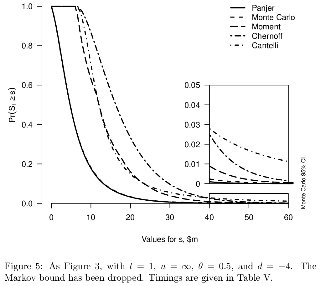
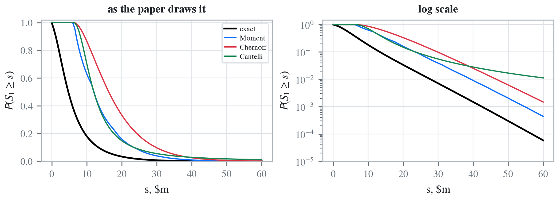
         'Figure 5': dict(t=1, theta=0.5, cap=np.inf, s=np.linspace(0, 60, 101) * M,
                          points=np.array([20, 40, 60]) * M),
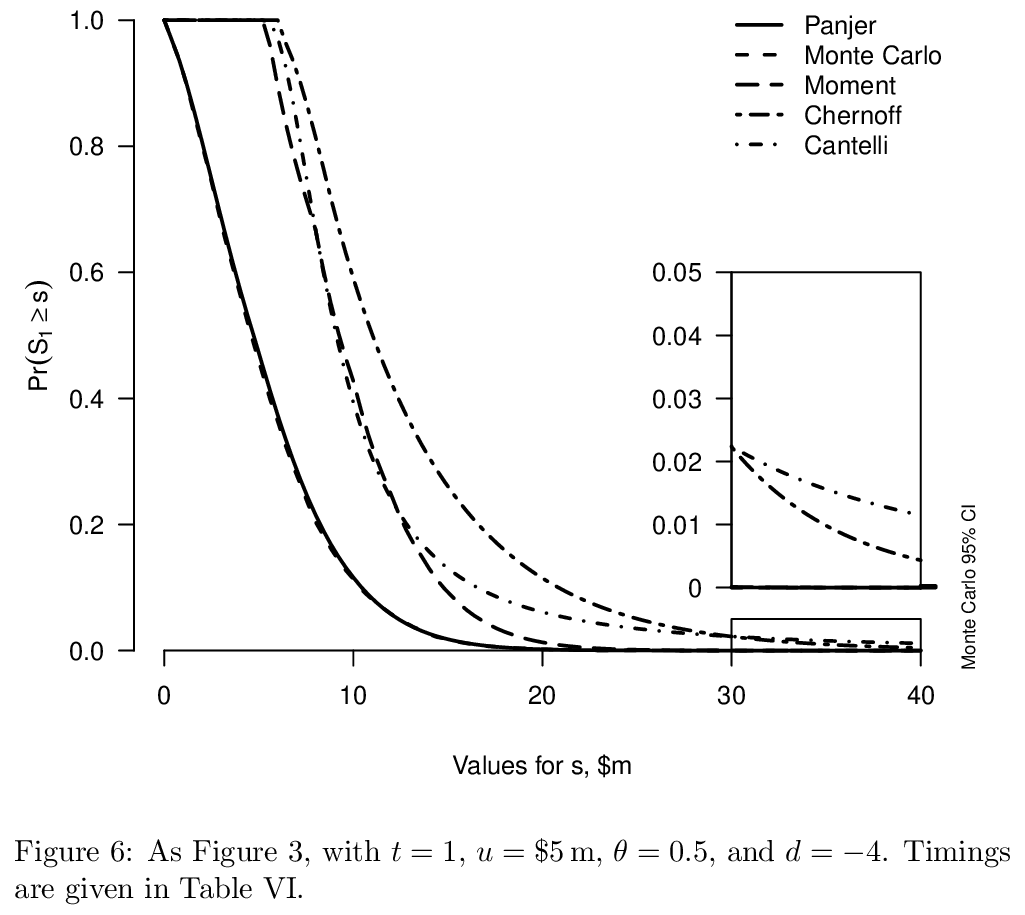
         'Figure 6': dict(t=1, theta=0.5, cap=5 * M, s=np.linspace(0, 40, 101) * M,
                          points=S3),
         'Figure 7': dict(t=10, theta=0.5, cap=5 * M, s=np.linspace(0, 120, 101) * M,
                          points=np.array([60, 90, 120]) * M)}
EXACT_CASE = {'Figure 3': H}
case = CASES['Figure 3']
case_figure(case['s'], {'exact': exceed(H, case['s']),
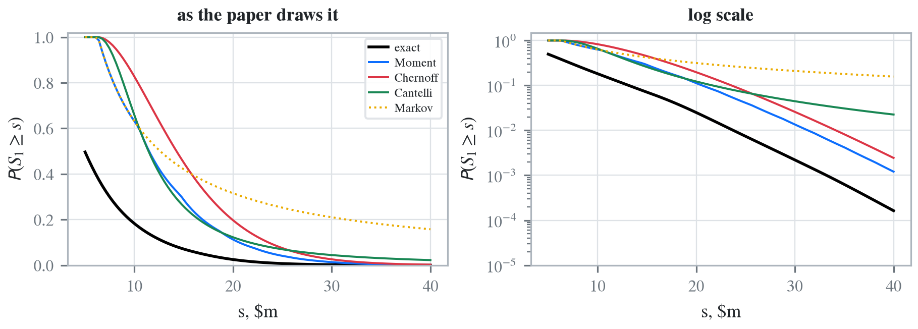
                        **bounds(T4, case['s'], case['t'], case['theta'], case['cap'])});

Figure 5: Reproducing Figure 3: fixed losses, \(t = 1\), no cap, bounds at \(d = -4\), against the exact uncompressed probability. Left as the paper draws it, right on a log scale.

Figure 5 shows what the paper’s linear axis cannot. The moment and Chernoff curves do approach the exact curve on a linear axis, because all three approach zero. On the log scale they run parallel to it at several times its value, and the gap widens as \(s\) grows: Table 11, after the four figures, has the moment bound 4.5 times the exact value at $20m and 7.4 times at $40m, and the Chernoff bound nearly twice the moment bound. The moment bound’s best \(k\) is 4 at $20m and 10 at $40m, far inside a search that runs to 200, so the gap is a property of the bound and not of where the search stopped. Likewise the optimal \(v\) for fixed losses lies inside the authors’ range, so their Chernoff curve here is the Chernoff bound.

3.6 Gamma event losses: Figure 5

Figure 6 makes each event’s loss gamma with its tabulated loss as the mean and a coefficient of variation of 0.5. There is no closed form for the exact distribution, but it is easy to compute: the severity is the rate weighted mixture of 1,145 gammas at \(d = -4\), each discretized to $10,000 buckets from its distribution function, and aggregate convolves the mixture as it would any other severity. Under a 50% coefficient of variation the $10,000 rounding of the means is invisible, as Table 9 shows by repeating the calculation at \(d = -3\), so the table compressed to $10,000 serves as the exact reference whenever losses are gamma.

Figure 6: Gollini and Rougier (2016), Figure 5.

S5 = CASES['Figure 5']['points']
start = time.perf_counter()
G3 = gamma_aggregate(TABLES[-3], 1e4, 15)
G3_SECONDS = time.perf_counter() - start
check = pd.DataFrame({'s, $m': S5 / M, 'd = -4': exceed(G4, S5),
                      'd = -3': exceed(G3, S5)})
check['rel err'] = check['d = -4'] / check['d = -3'] - 1
GT(check.set_index('s, $m'), formatters={'d = -4': '{x:.4e}', 'd = -3': '{x:.4e}'})

Table 9: Gamma losses with a coefficient of variation of 0.5: \(\mathsf P(S_1 \ge s)\) computed on the table compressed to $10,000 and to $1,000, with the seconds each took.

s, $m	d = -4	d = -3	rel err
20	3.3568e-02	3.3568e-02	1.25e-05
40	1.4745e-03	1.4743e-03	1.33e-04
60	5.8163e-05	5.8150e-05	2.27e-04

The two compressions in Table 9 agree to better than 0.03% at every \(s\); the \(d = -4\) build took about a second and the \(d = -3\) build a few. Figure 7 reproduces Figure 5. The authors drop the Markov bound from here on.

EXACT_CASE['Figure 5'] = G4
case = CASES['Figure 5']
case_figure(case['s'], {'exact': exceed(G4, case['s']),
                        **bounds(T4, case['s'], case['t'], case['theta'], case['cap'])});

Figure 7: Reproducing Figure 5: gamma losses with a coefficient of variation of 0.5, \(t = 1\), no cap, bounds at \(d = -4\). Left as the paper draws it, right on a log scale.

In Figure 7 the moment bound is between 4.8 and 7.6 times the exact value from $20m to $60m. The Chernoff bound is further off than with fixed losses, because the gamma MGF of the largest event is infinite at \(v = \beta_i\), so the search must stop at \(\min_i \beta_i\), about 0.16 per $m, which is short of where the bound would like to go.

3.7 Capped gamma losses: Figures 6 and 7

Figure 8 caps each event’s loss at $5m, and Figure 10 runs the same model over ten years. The exact distribution comes from the same construction with the mass above $5m moved to the bucket at $5m, and ten years multiply the event rate by ten.

Figure 8: Gollini and Rougier (2016), Figure 6.

V_FREE = np.linspace(0, 1.5, 3001)       # per $m; the capped MGF is finite everywhere
CAPPED_SECONDS = {}
for name in ('Figure 6', 'Figure 7'):
    case = CASES[name]
    start = time.perf_counter()
    EXACT_CASE[name] = gamma_aggregate(T4, 1e4, 15 if case['t'] == 1 else 16,
                                       t=case['t'], cap=case['cap'])
    CAPPED_SECONDS[name] = time.perf_counter() - start


def capped_curves(name):
    """The exact curve, the paper's bounds, and the unrestricted Chernoff bound."""
    case = CASES[name]
    model = dict(t=case['t'], theta=case['theta'], cap=case['cap'])
    return {'exact': exceed(EXACT_CASE[name], case['s']),
            **bounds(T4, case['s'], **model),
            'Chernoff, unrestricted': chernoff(T4, case['s'], V_FREE, interior=True,
                                               **model)}


case_figure(CASES['Figure 6']['s'], capped_curves('Figure 6'), floor=1e-9);

Figure 9: Reproducing Figure 6: gamma losses capped at $5m, \(t = 1\), bounds at \(d = -4\), with the Chernoff bound also over an unrestricted range of \(v\). Left as the paper draws it, right on a log scale.

Figure 10: Gollini and Rougier (2016), Figure 7.

case_figure(CASES['Figure 7']['s'], capped_curves('Figure 7'), t=10, floor=1e-7);

Figure 11: Reproducing Figure 7: gamma losses capped at $5m, \(t = 10\), bounds at \(d = -4\), with the Chernoff bound also over an unrestricted range of \(v\). Left as the paper draws it, right on a log scale.

The cap changes the Chernoff bound. A capped loss is bounded, so its MGF is finite for every \(v\), but the authors keep the search range of the uncapped gamma, \(v < \min_i \beta_i\). Their Appendix gives that range for the gamma, and it was not revisited for the cap. Figure 9 and Figure 11 show the Chernoff bound both ways, and Table 10 gives the values at three points. At $40m in one year the bound over the authors’ range is 0.0043 and the bound over all \(v\) is \(7.1 \times 10^{-7}\), against an exact probability of \(3.6 \times 10^{-8}\): the Chernoff curve in Figure 6 is not the Chernoff bound, and it is looser by a factor of about 6,000. Over all \(v\) the Chernoff bound lies between one and two times the moment bound, which is the order the authors cite from Philips and Nelson (1995): optimized over its full range, the moment bound is never worse than the Chernoff bound.

rows = []
for name in ('Figure 6', 'Figure 7'):
    case = CASES[name]
    model = dict(t=case['t'], theta=case['theta'], cap=case['cap'])
    s = case['points']
    rows.append(pd.DataFrame({
        'case': name, 't': case['t'], 's, $m': s / M,
        'exact': exceed(EXACT_CASE[name], s),
        'moment': moment_bound(T4, s, **model),
        'Chernoff, paper': chernoff(T4, s, paper_v(T4, 0.5, case['cap']), **model),
        'Chernoff, all v': chernoff(T4, s, V_FREE, interior=True, **model)}))
chern = pd.concat(rows).set_index(['case', 't', 's, $m'])
GT(chern, float_format='{x:.3e}')

Table 10: Capped gamma losses: the Chernoff bound over the authors’ range of \(v\) and over all \(v\), beside the moment bound and the exact probability.

case	t	s, $m	exact	moment	Chernoff, paper	Chernoff, all v
Figure 6	1	20	2.071e-03	1.310e-02	1.147e-01	2.118e-02
		30	1.241e-05	1.065e-04	2.229e-02	1.888e-04
		40	3.571e-08	3.788e-07	4.330e-03	7.079e-07
Figure 7	10	60	2.847e-01	8.232e-01	8.736e-01	8.736e-01
		90	2.965e-03	2.024e-02	2.649e-02	2.539e-02
		120	1.861e-06	1.920e-05	1.943e-04	2.659e-05

Table 11 collects the four cases at three or four points each, every bound as a multiple of the exact probability. The paper’s linear axes show none of these multiples. A factor of 7 at a probability of 0.0002 is a gap of a millimeter on a page whose vertical axis runs from 0 to 1.

rows = []
for name, case in CASES.items():
    s = case['points']
    ex = exceed(EXACT_CASE[name], s)
    b = bounds(T4, s, case['t'], case['theta'], case['cap'])
    k = moment_bound(T4, s, case['t'], case['theta'], case['cap'], argmin=True)[1]
    rows.append(pd.DataFrame({'case': name, 's, $m': s / M, 'exact': ex,
                              'Moment': b['Moment'] / ex, 'k': k,
                              'Chernoff': b['Chernoff'] / ex,
                              'Cantelli': b['Cantelli'] / ex}))
GT(pd.concat(rows).set_index(['case', 's, $m']),
   formatters={'exact': '{x:.3e}', 'Moment': 2, 'k': '{x:.0f}', 'Chernoff': 2,
               'Cantelli': 2})

Table 11: The exact probability for each of the paper’s four cases, each bound as a multiple of it, and the \(k\) that minimizes the moment bound. The Chernoff bound is over the authors’ range of \(v\).

case	s, $m	exact	Moment	k	Chernoff	Cantelli
Figure 3	10	1.827e-01	3.45	1	4.53	3.60
	20	2.496e-02	4.51	4	7.89	4.91
	30	2.200e-03	6.15	7	11.73	20.25
	40	1.633e-04	7.39	10	14.94	138.07
Figure 5	20	3.357e-02	4.78	3	9.95	4.43
	40	1.475e-03	6.11	6	17.10	19.00
	60	5.816e-05	7.57	9	25.31	192.99
Figure 6	20	2.071e-03	6.32	9	55.40	29.45
	30	1.241e-05	8.58	16	1,796.11	1,805.06
	40	3.571e-08	10.61	24	121,278.92	320,873.94
Figure 7	60	2.847e-01	2.89	3	3.07	2.73
	90	2.965e-03	6.83	17	8.93	32.19
	120	1.861e-06	10.31	33	104.36	16,469.22

3.8 Figure 1 and the Monte Carlo sample size

Figure 12 is a design calculation for Monte Carlo. Let \(u_{0.95}(x; n)\) be the upper limit of the 95% Jeffreys interval for a probability, which the authors take from Brown et al. (2001), after \(x\) exceedances in \(n\) draws: the 0.975 quantile of a beta distribution with parameters \(x + 1/2\) and \(n - x + 1/2\). The figure plots \(\mathsf P\{u_{0.95}(X; n) \le \kappa_0\}\) for \(X\) binomial with \(n\) trials and probability \(p_0 = \kappa_0/2\), so that it gives the chance that a simulation of size \(n\) demonstrates, with 95% confidence, a probability that is in fact half the regulatory limit. The calculation is exact and needs no simulation: for each \(x\), find the smallest \(n\) at which \(u_{0.95}(x; n) \le \kappa_0\), and sum the binomial probabilities of the \(x\) that qualify.

Figure 12: Gollini and Rougier (2016), Figure 1.

def design_probability(ns, p0, kappa=0.005, level=0.95):
    """Pr{u(X; n) <= kappa}, X ~ Binomial(n, p0), at every n in ns.

    u(x; n) falls as n grows, so each x qualifies from a first n onward; the
    largest qualifying x at n is found by search, and the answer is a binomial
    distribution function.
    """
    q = (1 + level) / 2
    first = []
    for x in range(int(ns.max() * kappa) + 2):
        lo, hi = x + 1, 10 * ns.max()
        while lo < hi:
            mid = (lo + hi) // 2
            if stats.beta.ppf(q, x + 0.5, mid - x + 0.5) <= kappa:
                hi = mid
            else:
                lo = mid + 1
        first.append(lo)
    xstar = np.searchsorted(np.array(first), ns, side='right') - 1
    return np.where(xstar >= 0, stats.binom.cdf(xstar, ns, p0), 0.0)


KAPPA = 0.005
NS = np.unique(np.round(np.logspace(3, 5, 2000)).astype(int))
fig, ax = figure('three-quarter')
ax.semilogx(NS, design_probability(NS, KAPPA / 2), lw=0.6, c='k')
ax.axvline(1e4, c='k', lw=0.6, ls=':')
ax.set(xlabel='size of Monte Carlo sample, n',
       ylabel=r'$\mathsf{P}\{u_{0.95}(X; n) \leq \kappa_0\}$', ylim=(0, 1.02));

Figure 13: Reproducing Figure 1, at about 2,000 values of \(n\) from 1,000 to 100,000, evenly spaced on the log scale: the probability that the upper limit of the 95% Jeffreys interval is at most \(\kappa_0 = 0.005\) when \(p_0 = \kappa_0 / 2\). The paper’s axis stops at the dotted line.

Figure 13 matches the paper’s curve, 0.29 at \(n = 1{,}000\) and 0.986 at \(n = 10{,}000\), and the saw teeth are the discreteness of \(X\). Beyond \(10^4\) the probability is within \(10^{-4}\) of one by \(n = 20{,}000\). The paper’s figure therefore shows that \(10^4\) draws already suffice, which is also the conclusion of the authors’ summary, “10,000 Monte Carlo simulations should suffice”. Beside the figure, though, they write that “\(n = 10^5\) seems to be a good choice”, and in Section 6.2 they report using \(10^5\). Their script calls the simulation with the package default, nsim = 10e3, which is \(10^4\), so the figures were drawn from \(10^4\) draws, not the \(10^5\) reported in the text.

The design is for a probability of \(\kappa_0/2\). At the point where the figures draw their Monte Carlo interval, \(s_0 = \$40\)m, the probability is far smaller, and Table 12 shows what that means for the interval.

P40 = EXACT[-1]
mc = []
for n in (10 ** 3, 10 ** 4, 10 ** 5):
    x = round(n * P40)
    lo, hi = stats.beta.ppf([0.025, 0.975], x + 0.5, n - x + 0.5)
    mc.append({'n': n, 'design probability': design_probability(np.array([n]), KAPPA / 2)[0],
               'expected exceedances': n * P40, 'x': x,
               'Jeffreys lower': lo if x > 0 else 0.0, 'Jeffreys upper': hi,
               'exact': P40})
GT(pd.DataFrame(mc).set_index('n'),
   formatters={'n': '{x:,.0f}', 'design probability': 4, 'expected exceedances': 2,
               'x': '{x:,.0f}', 'Jeffreys lower': '{x:.2e}', 'Jeffreys upper': '{x:.2e}',
               'exact': '{x:.2e}'})

Table 12: Monte Carlo at $40m with fixed losses: the expected number of exceedances, and the 95% Jeffreys interval at that count, against the exact probability, with the design probability of Figure 1.

n	design probability	expected exceedances	x	Jeffreys lower	Jeffreys upper	exact
1,000	0.2869	0.16	0	0.00e+00	2.51e-03	1.63e-04
10,000	0.9856	1.63	2	4.16e-05	6.41e-04	1.63e-04
100,000	1.0000	16.33	16	9.52e-05	2.54e-04	1.63e-04

With \(10^4\) draws the expected number of exceedances at $40m is 1.6, and the interval at two exceedances in Table 12 spans a factor of fifteen. The small count is no criticism of the design, which addresses a different question, but it does mean that the right end of the Monte Carlo curves in Figures 3, 5, 6 and 7 rests on a handful of draws.

3.9 Timings

Tables IV to VII, Figure 14 to Figure 17, give the time each method took on each compression for Figures 3, 5, 6 and 7. The Panjer recursion is the only method whose time grows quickly with the table, and the authors stopped it at \(d = -2\) for Figure 3 and at \(d = -3\) for the others.

Figure 14: Gollini and Rougier (2016), Table IV.

Figure 15: Gollini and Rougier (2016), Table V.

Figure 16: Gollini and Rougier (2016), Table VI.

Figure 17: Gollini and Rougier (2016), Table VII.

Table 13 sets the paper’s Panjer times beside the time aggregate took for each exact reference in this chapter, measured when the book was rendered: the full table at a $10 bucket for fixed losses, and the gamma mixture at \(d = -4\) for the others, including the construction of the severity. The seconds are on different machines a decade apart, so the ratios matter less than the structure. The FFT computes a compound distribution with two transforms whatever the size of the table, and the size of the table enters only through the severity, once.

GT(pd.DataFrame([
    ('Figure 3', 0.461, -2, 4651.298, 'full table, $10 bucket', H_SECONDS),
    ('Figure 5', 1.509, -3, 121.062, 'd = -4, gamma, $10,000 bucket', G4_SECONDS),
    ('Figure 6', 0.275, -3, 11.950, 'd = -4, capped gamma', CAPPED_SECONDS['Figure 6']),
    ('Figure 7', 0.587, -3, 46.000, 'd = -4, capped gamma, ten years',
     CAPPED_SECONDS['Figure 7']),
], columns=['case', 'Panjer, d = -4', 'finest d', 'Panjer, finest d', 'aggregate model',
            'aggregate seconds']).set_index('case'),
   formatters={'Panjer, d = -4': 3, 'finest d': '{x:.0f}', 'Panjer, finest d': '{x:,.3f}',
               'aggregate seconds': 3})

Table 13: The paper’s Panjer recursion at \(d = -4\) and at its finest compression, against aggregate building each exact reference in this chapter, in seconds.

case	Panjer, d = -4	finest d	Panjer, finest d	aggregate model	aggregate seconds
Figure 3	0.461	-2	4,651.298	full table, $10 bucket	0.793
Figure 5	1.509	-3	121.062	d = -4, gamma, $10,000 bucket	0.846
Figure 6	0.275	-3	11.950	d = -4, capped gamma	0.032
Figure 7	0.587	-3	46.000	d = -4, capped gamma, ten years	0.038

4 Comments

4.1 Reach of the exact computation

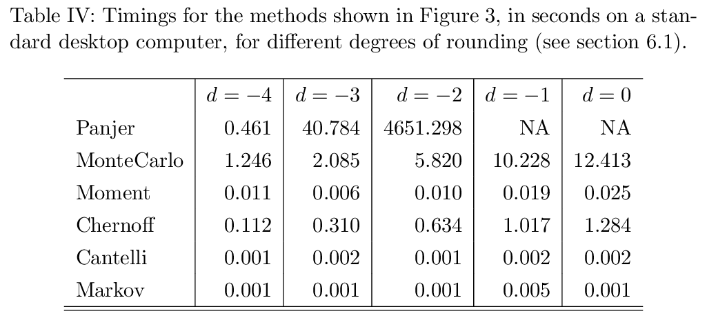
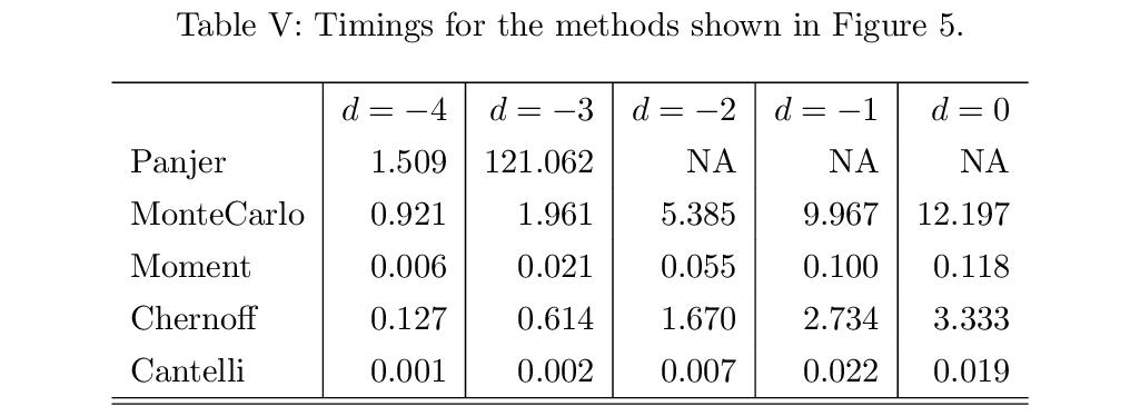
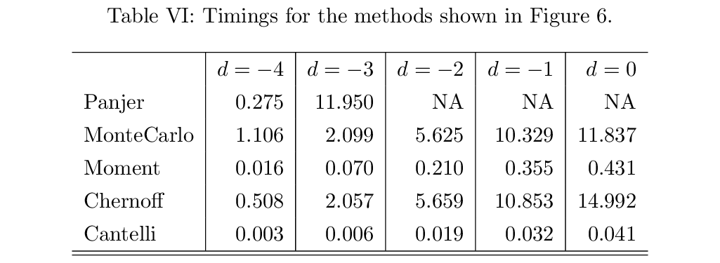
The authors’ case for bounds rests on exact methods being too slow without compression. On the evidence of Table 6 and Table 13 that premise no longer holds, and it did not hold in 2015 either: the FFT was as available then as now, and the reason it is fast is the structure of the compound Poisson, not the speed of the machine. The uncompressed table takes a fraction of a second at a $100 bucket, and the gamma version takes about a second. The bounds keep a use where only the moments of a table are known, or where a bound is needed in closed form inside some larger calculation, but as a substitute for computing the distribution of a table that is in hand they are not needed.

4.2 Looseness of the bounds

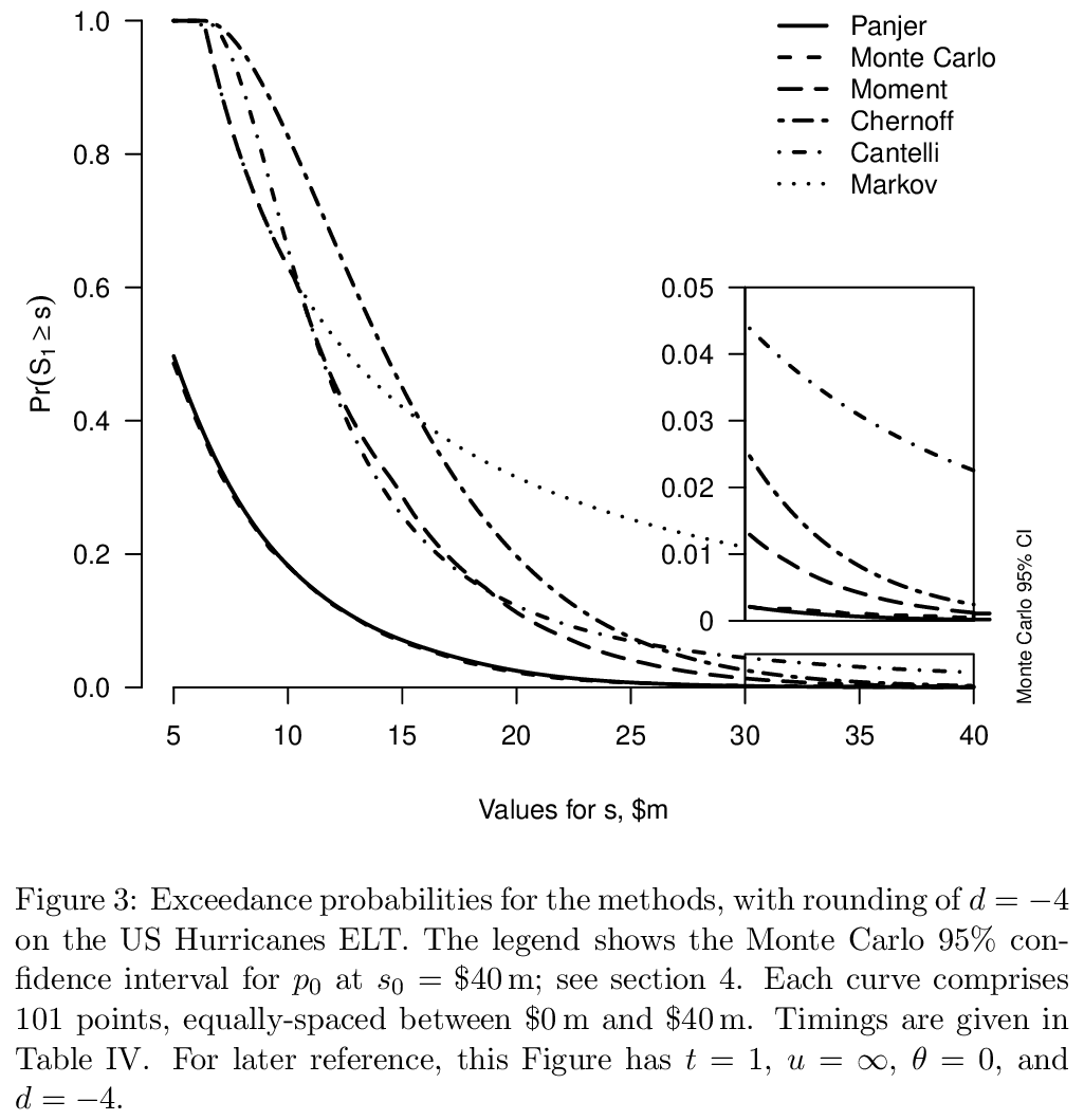
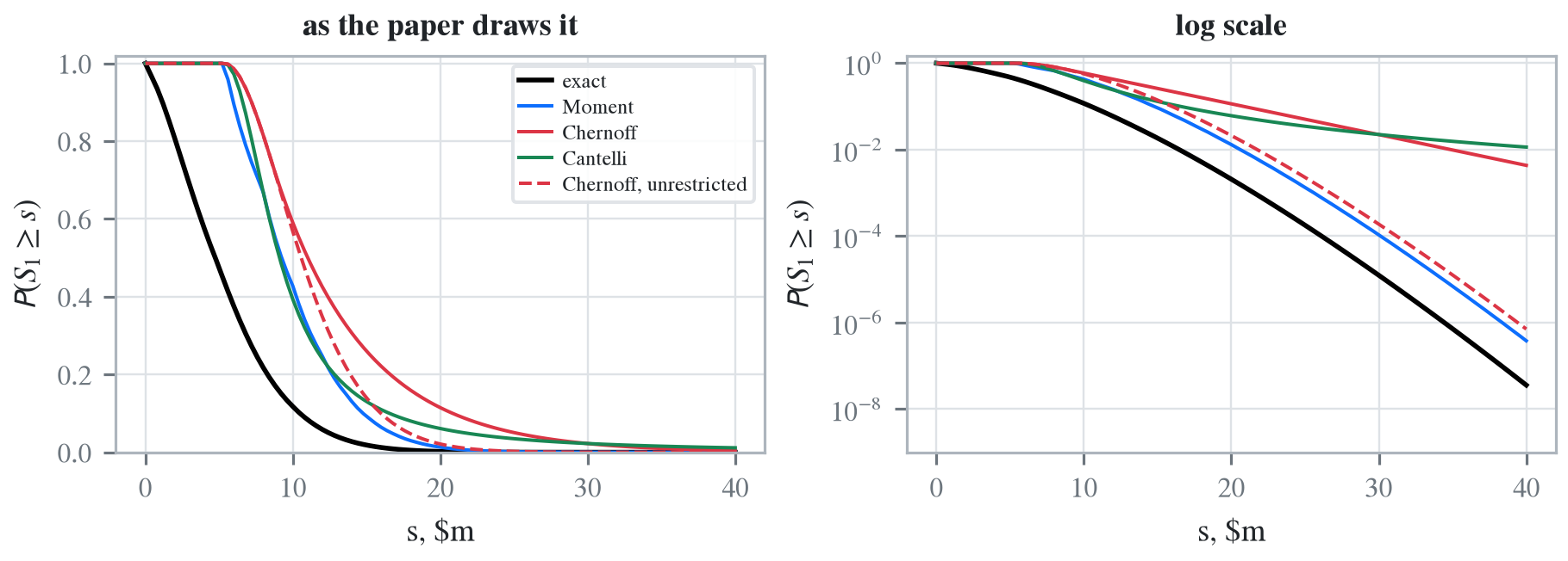
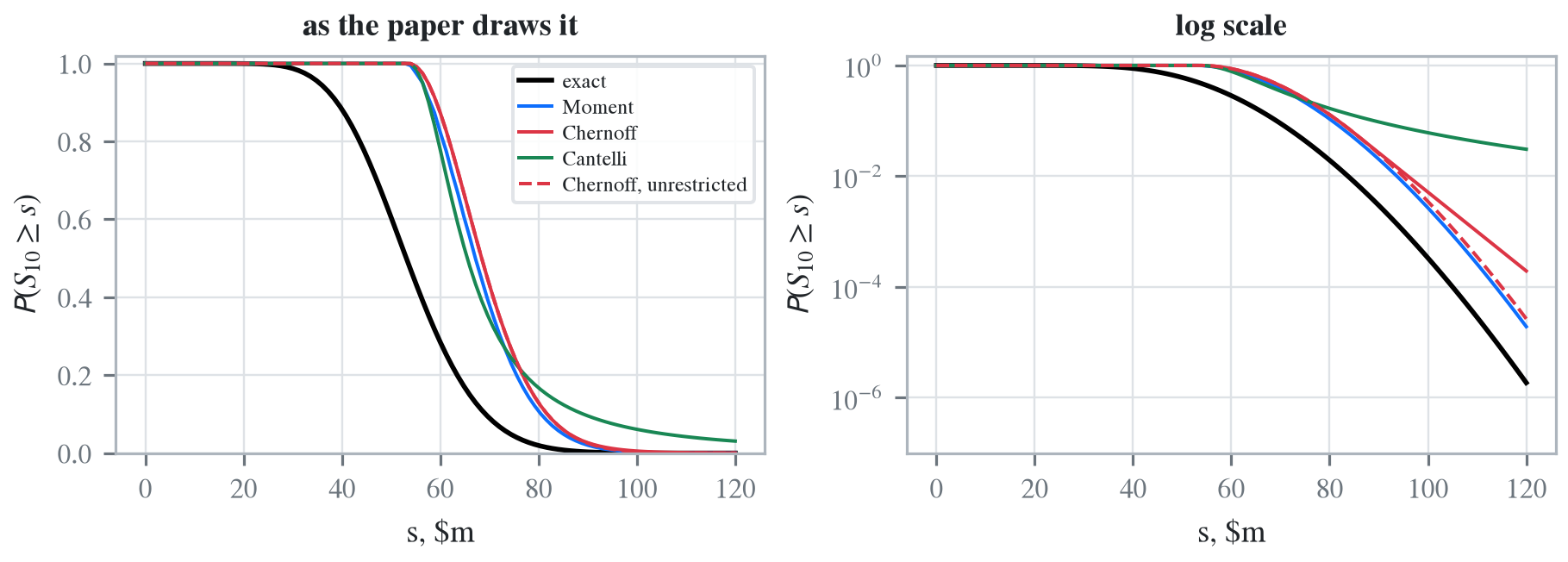
The exact 1-in-200 annual loss with fixed event losses is $26.6m. Table 14 gives, for each bound, the smallest capital \(s\) at which the bound falls to 0.005, which is the solvency question asked of the bound directly. On the full table the moment bound calls for 29% more capital than the exact answer, Chernoff for 39% more, and Cantelli for nearly three times as much. A regulator satisfied by a bound is satisfied at a cost, and the exact answer costs a second.

def chernoff_fixed(table, s, t=1):
    """The Chernoff bound for fixed losses at its exact optimum, and the optimal v.

    With fixed losses the MGF is finite everywhere and the optimum solves
    lambda t P[Y e^{vY}] = s, monotone in v.
    """
    x = table.Dollars.to_numpy() / M
    rate = table.Rate.to_numpy()
    out = []
    for s_m in np.atleast_1d(np.asarray(s, float)) / M:
        slope = lambda v: t * (rate * x * np.exp(v * x)).sum() - s_m
        if slope(0) >= 0:
            out.append((1.0, 0.0))
            continue
        hi = 1.0
        while slope(hi) < 0:
            hi *= 2
        v = optimize.brentq(slope, 0, hi, xtol=1e-14)
        out.append((np.exp(-v * s_m + t * (rate @ np.exp(v * x) - rate.sum())), v))
    return np.array(out).T


def quantile(a, p):
    """The p quantile of the distribution on the grid of `a`."""
    return a.xs[np.searchsorted(np.cumsum(a.agg_density), p)]


FULL = TABLES[0]
VAR = quantile(H, 0.995)
capital = {'exact': VAR}
for name, fn in (('moment', lambda s: moment_bound(FULL, [s])[0]),
                 ('Chernoff', lambda s: chernoff_fixed(FULL, [s])[0][0]),
                 ('Cantelli', lambda s: cantelli(FULL, [s])[0]),
                 ('Markov', lambda s: markov(FULL, [s])[0])):
    capital[name] = optimize.brentq(lambda s: fn(s) - 0.005, 10 * M, 1e4 * M, xtol=1e3)
GT(pd.DataFrame({'capital, $m': pd.Series(capital) / M,
                 'multiple of exact': pd.Series(capital) / VAR})
   .rename_axis('method'), formatters={'capital, $m': '{x:,.2f}', 'multiple of exact': 2})

Table 14: The capital each method requires for a 1-in-200 annual probability, fixed losses, full table, in millions of dollars and as a multiple of the exact value.

method	capital, $m	multiple of exact
exact	26.62	1.00
moment	34.25	1.29
Chernoff	37.07	1.39
Cantelli	78.49	2.95
Markov	1,261.88	47.41

4.3 Large deviations and the Chernoff bound

In Section 3 the authors argue from large deviations that “as \(t\) becomes large the Chernoff upper bound becomes exact”, and that, the moment bound being tighter, “both bounds are converging from above on the actual probability”. In Section 6.1 they rely on the argument to judge compression with the moment bound. The large deviations limit is a statement about the exponent: for a fixed loss per year \(a\) above the mean, \(t^{-1}\log \mathsf P(S_t \ge at) \to -I(a)\), and the Chernoff bound is \(e^{-tI(a)}\) exactly. The \(o(t)\) term in the authors’ display allows any factor that grows more slowly than an exponential. By the theorem of Bahadur and Rao (1960) the factor is \[ \frac{e^{-tI(a)}}{\mathsf P(S_t \ge at)} \sim v_a \sigma_a \sqrt{2\pi t}, \] where \(v_a\) is the optimal \(v\) and \(\sigma_a^2 = \lambda \mathsf P(Y^2 e^{v_a Y})\) is the annual variance under the tilted measure. The ratio of the bound to the probability grows like \(\sqrt t\); the bound is exact on a logarithmic scale and not otherwise. Table 15 shows the ratio at $15m a year on the full table with fixed losses, and the ratio follows the prediction ever more closely as \(t\) grows. The moment bound’s ratio grows too.

A_RATE = 15 * M
LOG2_BY_T = {1: 17, 2: 18, 4: 18, 8: 19, 16: 20}
x_m, rate = FULL.Dollars.to_numpy() / M, FULL.Rate.to_numpy()
ld = []
for t, log2 in LOG2_BY_T.items():
    s = A_RATE * t
    ex = exceed(elt_aggregate(ELT.Loss, ELT.Rate, 1e3, log2, t=t), s)[()]
    (ch,), (v,) = chernoff_fixed(FULL, [s], t)
    sigma = np.sqrt(rate @ (x_m ** 2 * np.exp(v * x_m)))
    ld.append({'t': t, 's, $m': s / M, 'exact': ex, 'Chernoff multiple': ch / ex,
               'predicted': v * sigma * np.sqrt(2 * np.pi * t),
               'moment multiple': moment_bound(FULL, [s], t=t)[0] / ex})
GT(pd.DataFrame(ld).set_index('t'),
   formatters={'s, $m': '{x:,.0f}', 'exact': '{x:.3e}', 'Chernoff multiple': 2,
               'predicted': 2, 'moment multiple': 2})

Table 15: Fixed losses, full table, at a loss of $15m a year over \(t\) years: the exact probability, each bound as a multiple of it, and the Bahadur and Rao prediction for the Chernoff multiple.

t	s, $m	exact	Chernoff multiple	predicted	moment multiple
1	15	7.093e-02	6.34	4.04	4.04
2	30	2.694e-02	7.51	5.72	4.91
4	60	4.324e-03	9.47	8.09	6.31
8	120	1.343e-04	12.48	11.44	8.38
16	240	1.657e-07	16.95	16.18	11.44

Holding the probability fixed instead of the loss per year gives the same answer by another route. At the 99.5% point of \(S_t\) the central limit theorem takes over as \(t\) grows, the Chernoff bound tends to \(e^{-z^2/2}\) with \(z\) the normal 99.5% point, and the ratio to 0.005 tends to 7.25, not to 1. Table 16 shows the ratio at one year and at ten on its way there.

z = stats.norm.ppf(0.995)
fl = []
for t, log2 in ((1, 17), (10, 18)):
    a = elt_aggregate(ELT.Loss, ELT.Rate, 1e3, log2, t=t)
    q = quantile(a, 0.995)
    ex = exceed(a, q)[()]
    fl.append({'t': str(t), 'VaR 99.5%, $m': q / M, 'exact': ex,
               'Chernoff multiple': chernoff_fixed(FULL, [q], t)[0][0] / ex,
               'moment multiple': moment_bound(FULL, [q], t=t)[0] / ex})
fl.append({'t': 'normal limit', 'VaR 99.5%, $m': np.nan, 'exact': 0.005,
           'Chernoff multiple': np.exp(-z * z / 2) / 0.005, 'moment multiple': np.nan})
GT(pd.DataFrame(fl).set_index('t'),
   formatters={'VaR 99.5%, $m': '{x:,.2f}', 'exact': 5, 'Chernoff multiple': 2,
               'moment multiple': 2})

Table 16: Fixed losses, full table, at the 99.5% point of \(S_t\): each bound as a multiple of the exact probability, at one and ten years and in the normal limit.

t	VaR 99.5%, $m	exact	Chernoff multiple	moment multiple
1	26.62	0.00500	10.73	5.77
10	112.45	0.00500	8.66	6.55
normal limit	—	0.00500	7.25	—

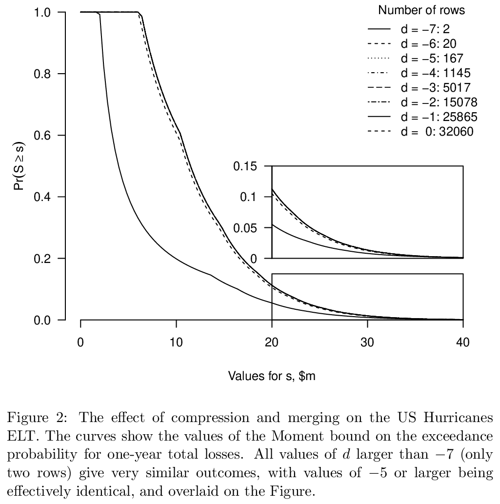
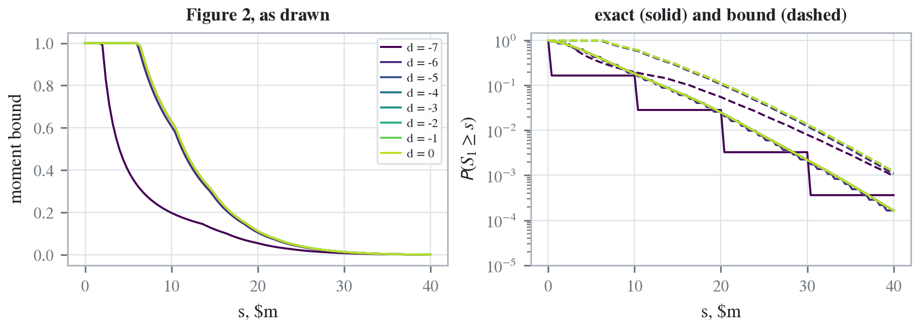
Neither limit is 1. The squeeze the authors describe does not occur, and a bound that is several times the probability at every horizon cannot serve as the yardstick for a compression error of a few percent, which is what Table 8 found.

4.4 The Monte Carlo sample size

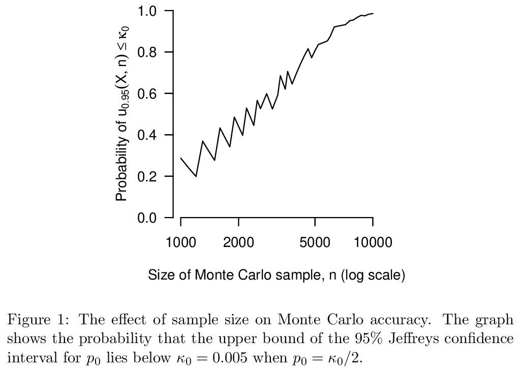
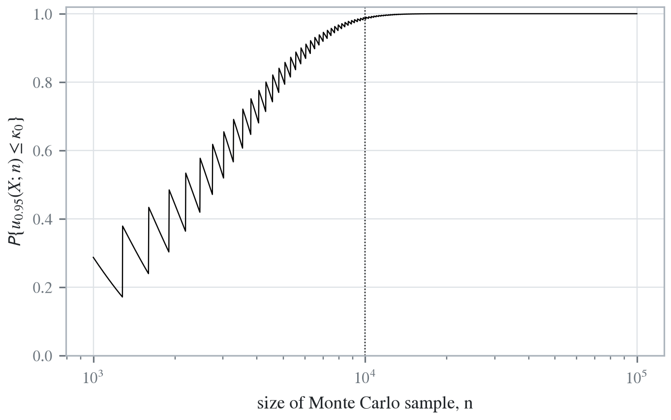
The authors give two sample sizes. In Section 4 and Section 6.2 they give \(10^5\). Figure 1 supports \(10^4\), the summary in Section 7 recommends 10,000, and the package default, from which the figures were drawn, is \(10^4\). On the authors’ own design calculation, Figure 13, \(10^4\) is the defensible choice, with a probability of 0.986, and \(10^5\) is ample. The inconsistency is in what the text reports: a sample ten times the one the figures were computed from.

4.5 The Monte Carlo time in Table VII

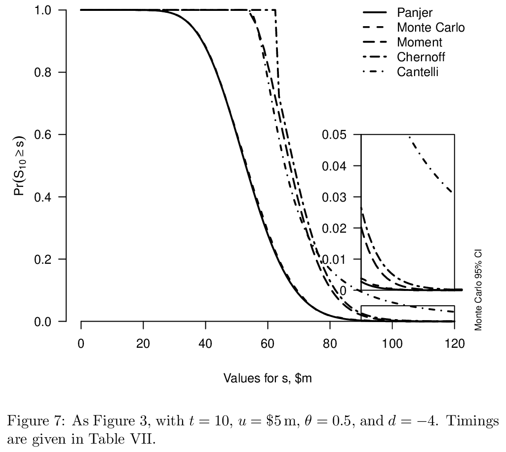
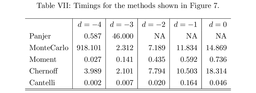
In Figure 17 Monte Carlo takes 918.101 seconds at \(d = -4\) and 2.312 seconds at \(d = -3\). Every other Monte Carlo time in the four tables is between 0.9 and 15 seconds and grows with the size of the table, as it should, since a simulation draws from the table. The value at \(d = -4\) is out of line by a factor of several hundred and is most likely an interruption during the run rather than a property of the method. A timing cannot be reproduced, so the point stays an observation.

4.6 The capped gamma and the DecL limit

The authors prefer a capped gamma to a beta scaled to \([0, u]\) because the cap leaves an atom at \(u\), which is what a maximum insured loss does, while a scaled beta has none. A DecL limit, 5 xs 0 in the Hurricane.Capped program, places exactly that atom on the severity, and aggregate applies it to any severity, the gamma mixture included. The cap also bounds the loss, which is what makes the MGF finite everywhere and the authors’ Chernoff range too narrow, as Table 10 showed.

4.7 Long vectors in DecL

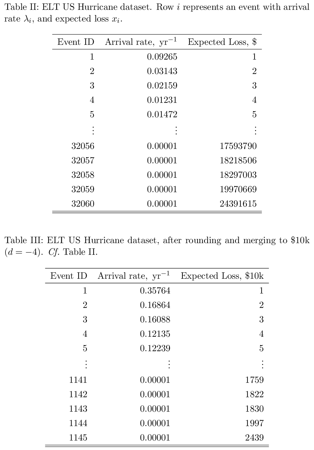
A DecL vector of 450 elements parses, and one of 500 exceeds Python’s recursion limit inside the parser, as Table 17 shows for the version of aggregate named in the preface. The full table, 32,060 rows, and even the table at \(d = -4\), 1,145 rows, are beyond that limit, which is why this chapter builds them through the Aggregate class. The division is a reasonable one in any case: a DecL program is a model a person writes and reads, and a table of thirty thousand rows is data, which belongs in a file and in the class, which accepts vectors of any length.

def parses(n):
    """Whether a dsev of n equally likely losses parses.

    The library's own build is used, not the book's recording one, so that the
    test programs stay out of the appendix.
    """
    vector = ' '.join(str(i + 1) for i in range(n))
    try:
        library_build(f'agg T 1 claim dsev [{vector}] fixed', update=False)
        return 'parses'
    except RecursionError:
        return 'RecursionError'


GT(pd.DataFrame({'n': [450, 500], 'result': [parses(450), parses(500)]}).set_index('n'),
   formatters={'n': '{x:,.0f}'})

Table 17: Parsing a dsev of n equally likely losses, on the version of aggregate named in the preface.

n	result
450	parses
500	RecursionError

Programs in the aggregate Loss Lab

Each program below opens in the aggregate Loss Lab, which builds it with nothing to install. The names are those in reproductions.agg, where every program is renamed by its paper’s citation key.

• Gollini2016.Hurricane: the US hurricane event loss table merged to $1m, 20 rows.
• Gollini2016.Hurricane.Capped: the same table with each event loss capped at $5m.
• Gollini2016.Hurricane.Gamma: the same table with each event loss gamma, coefficient of variation 0.5.

Bahadur, R. R., & Rao, R. R. (1960). On deviations of the sample mean. The Annals of Mathematical Statistics, 31(4), 1015–1027.

Brown, L. D., Cai, T. T., & DasGupta, A. (2001). Interval Estimation for a Binomial Proportion. Statistical Science. https://doi.org/10.1214/ss/1009213286

Gollini, I., & Rougier, J. (2016). Rapidly bounding the exceedance probabilities of high aggregate losses. The Journal of Operational Risk, 1–33. https://doi.org/10.21314/JOP.2016.179

Philips, T. K., & Nelson, R. (1995). The Moment Bound is Tighter than Chernoff’s Bound for Positive Tail Probabilities. The American Statistician. https://doi.org/10.1080/00031305.1995.10476137