Ben Rached, Hoel and Meo on the FFT accuracy floor
Reproducing Ben Rached, Hoel and Meo (2024), and testing its central claim against aggregate
Author
Stephen J. Mildenhall
Published
2026-10-22 19:55 commit b5ca906+
1 Introduction
Ben Rached et al. (2024) is a paper about aggregate’s FFT-based method, and its central claim is a criticism of it.
The authors compute \(\alpha = \mathsf P(\sum_{i=1}^n X_i < \gamma)\) for small \(\gamma\) by discretizing the severity density on a uniform mesh and convolving it \(n\) times. That is what aggregate does. The difference is the convolution: they use direct summation, and they argue, with a theorem and with numerical evidence, that using the FFT instead loses relative accuracy in the deep left tail.
We further compare direct-based convolution to FFT-based convolution, and show by formal theoretical arguments and in numerical experiments that FFT-based convolution is more sensitive to rounding errors and a less reliable method when the magnitude of the probability of failure is sufficiently small.
Their Lemma 4 and Theorem 3 make this quantitative. The FFT error is bounded in absolute terms, proportional to machine epsilon times the total mass, whereas direct convolution admits a relative bound, because summing and multiplying non-negative floating point numbers never cancels:
when \(\alpha \ll 1\), the result indicates that for a given resolution \(N\), the relative error may be substantially smaller for direct-based convolution than for FFT-based convolution.
So this example has two jobs. First, to reproduce what the paper publishes. And second, take the criticism seriously and find out exactly where aggregate stops working.
2 What is reproducible
Three published tables carry values rather than convergence rates.
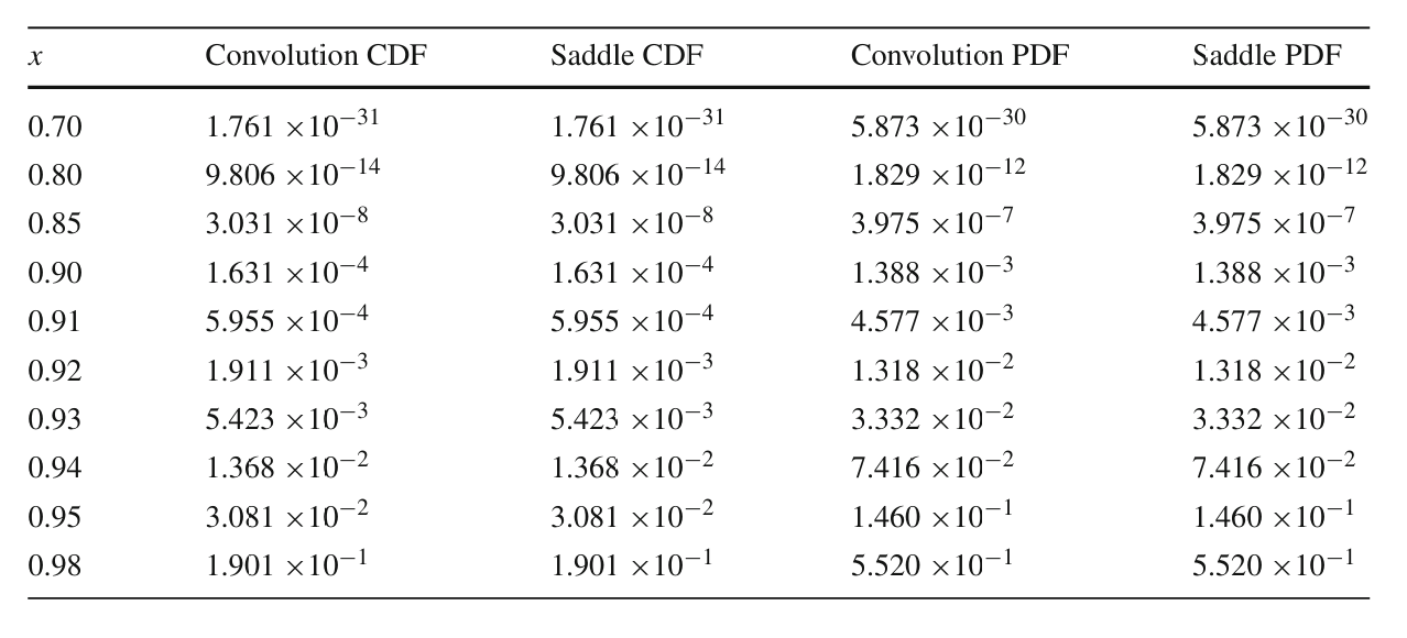
Table 6, Figure 1: CDF and PDF of \(S_{16}\) for \(X_i \sim \mathrm{LN}(0, 0.125^2)\), ten values of \(x\) with \(\gamma = 16x\), quoted to four significant figures, computed two independent ways (their convolution method and their implementation of the saddlepoint method of Asmussen et al. (2016)) which agree.
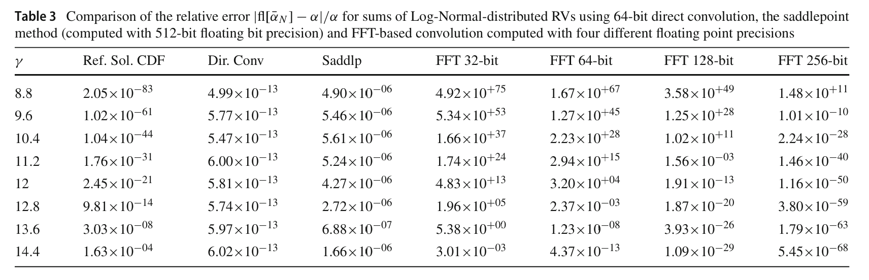
Table 3, Figure 2: a reference solution column for the same distribution, computed at 512-bit precision, spanning \(\alpha\) from \(1.63 \times 10^{-4}\) down to \(2.05 \times 10^{-83}\), alongside the measured relative error of 64-bit direct convolution and of FFT at four precisions.
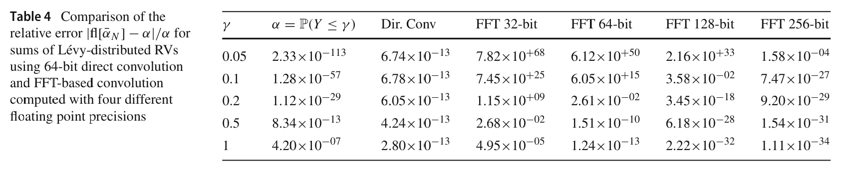
Table 4, Figure 3: the same for Lévy summands, where the exact answer is known in closed form because the Lévy distribution is stable.
Figures 1 to 5 are convergence plots and are not reproduced here.
3 Setup
%xmode minimalimport numpy as npimport pandas as pdfrom functools import partialfrom bookstyle import GT, build# Tail probabilities and relative errors read as powers of ten, not SI prefixes.GT = partial(GT, eng_style='exp')from scipy.special import erfcdef lognormal_sum(n, sigma, log2=22, bs=2.0**-13):return build(f'agg S dfreq [{n}] sev 1 * lognorm {sigma}', log2=log2, bs=bs, normalize=False)S16 = lognormal_sum(16, 0.125)print(f'E[S_16] from agg {S16.est_m:.10f}')print(f'E[S_16] exact {16* np.exp(0.125**2/2):.10f}')
The problem is \(\alpha = F_Y(\gamma)\) with \(\gamma = 16x\), \(Y = \sum_{i=1}^{16} X_i\), \(X_i \sim \mathrm{LN}(0, \sigma^2)\) and \(\sigma = 0.125\). The paper notes a caveat on its own saddlepoint column:
Note that the values calculated with our implementation of the saddlepoint method gives slightly different values compared with the values listed in the paper (Asmussen et al. 2016) (\(\pm 1\) in the third digit of the significand).
Figure 1: Ben Rached, Hoel and Meo (2024), Table 6, approximations of the CDF and PDF of \(Y\).
Table 1: Table 6, the CDF and PDF of \(S_{16}\) at ten thresholds, against the published values.
x
gamma
paper CDF
agg CDF
CDF rel err
paper PDF
agg PDF
PDF rel err
0.70000
11.20
176.100e-33
-49.396e-18
2.80e+14
5.873e-30
-4.018e-18
6.84e+11
0.80000
12.80
98.060e-15
98.010e-15
5.06e-04
1.829e-12
1.829e-12
2.67e-04
0.85000
13.60
30.310e-09
30.325e-09
4.89e-04
397.500e-09
397.542e-09
1.05e-04
0.90000
14.40
163.100e-06
163.093e-06
4.26e-05
1.388e-03
1.388e-03
2.63e-04
0.91000
14.56
595.500e-06
595.518e-06
2.97e-05
4.577e-03
4.577e-03
6.05e-05
0.92000
14.72
1.911e-03
1.912e-03
4.75e-04
13.180e-03
13.185e-03
3.73e-04
0.93000
14.88
5.423e-03
5.422e-03
2.60e-04
33.320e-03
33.319e-03
3.22e-05
0.94000
15.04
13.680e-03
13.674e-03
4.61e-04
74.160e-03
74.160e-03
4.58e-06
0.95000
15.20
30.810e-03
30.814e-03
1.35e-04
146.000e-03
145.958e-03
2.89e-04
0.98000
15.68
190.100e-03
190.099e-03
5.31e-06
552.000e-03
552.043e-03
7.81e-05
In Table 1 nine of the ten rows reproduce to between \(5 \times 10^{-6}\) and \(1.2 \times 10^{-3}\) relative, in both the CDF and the PDF. Since the paper quotes four significant figures, that is agreement to the last published digit almost everywhere.
The first row fails completely. The target is \(1.761 \times 10^{-31}\) and aggregate returns \(3.4 \times 10^{-17}\), wrong by fourteen orders of magnitude. That is precisely the effect the paper was written about, and the next section measures it.
5 Table 3: locating the floor
Table 3 is the experiment that motivates the paper. The reference solution is computed with 512-bit arithmetic, and the other columns give relative error for 64-bit direct convolution and for FFT at 32, 64, 128 and 256 bits. The published 64-bit FFT column is reproduced here so that aggregate can be placed against it.
Figure 2: Ben Rached, Hoel and Meo (2024), Table 3.
Table 2: Table 3, the 512-bit reference solution against the library and the paper’s own 64-bit FFT, in relative and absolute terms.
gamma
reference
agg
agg rel err
agg abs err
paper FFT64 rel err
paper FFT64 abs err
8.80
20.500e-84
30.241e-18
1.48e+66
3.02e-17
1.67e+67
3.42e-16
9.60
102.000e-63
22.145e-18
2.17e+44
2.21e-17
1.27e+45
1.30e-16
10.40
10.400e-45
-19.935e-18
1.92e+27
1.99e-17
2.23e+28
2.32e-16
11.20
176.000e-33
-49.396e-18
2.81e+14
4.94e-17
2.94e+15
5.17e-16
12.00
2.450e-21
-41.301e-18
1.69e+04
4.13e-17
3.20e+04
7.84e-17
12.80
98.100e-15
98.010e-15
9.13e-04
8.96e-17
2.37e-03
2.32e-16
13.60
30.300e-09
30.325e-09
8.19e-04
2.48e-11
1.23e-08
3.73e-16
14.40
163.000e-06
163.093e-06
5.71e-04
9.31e-08
4.37e-13
7.12e-17
Read the last two columns of Table 2 together. The paper’s own 64-bit FFT has a relative error that explodes as \(\gamma\) falls, from \(4 \times 10^{-13}\) to \(1.7 \times 10^{67}\), but its absolute error never leaves the band \(7 \times 10^{-17}\) to \(5 \times 10^{-16}\). aggregate shows the identical signature, with an absolute error pinned between \(9 \times 10^{-18}\) and \(7 \times 10^{-17}\) on every row where the target is smaller than that. The two implementations differ in almost every detail, and they land on the same wall, because the wall is machine epsilon and not the implementation.
The \(\gamma = 12\) row is the sharpest single check. The paper’s FFT64 relative error is \(3.20 \times 10^{4}\) against a reference of \(2.45 \times 10^{-21}\), implying an absolute error of \(7.8 \times 10^{-17}\). aggregate returns \(7.07 \times 10^{-17}\) where the true answer is \(2.45 \times 10^{-21}\), so its absolute error is also \(7.07 \times 10^{-17}\). Two unrelated FFT codes agreeing to 10% on the magnitude of their own roundoff noise is a strong confirmation of Theorem 3.
5.1 The floor does not move
If this were a resolution problem, refining the grid would fix it. Table 3 shows it is not.
Table 3: Three probabilities across four grid settings, showing which are stable under refinement and which are noise.
log2
bs
padding
F(12.0) [true 2.45e-21]
F(12.8) [true 9.81e-14]
F(14.4) [true 1.63e-04]
22
2^-13
1
-41.301e-18
98.010e-15
163.093e-06
22
2^-13
2
-81.443e-18
97.993e-15
163.093e-06
23
2^-13
2
-99.080e-18
97.955e-15
163.093e-06
24
2^-14
2
16.561e-18
98.126e-15
163.135e-06
In Table 3, across a factor of four in resolution and both padding settings, F(12.0) wanders between \(-8.4 \times 10^{-17}\) and \(+1.0 \times 10^{-16}\), changing sign. A quantity that flips sign under refinement is not converging to anything; it is noise. Meanwhile F(12.8) is stable to three figures and F(14.4) to six.
So the operating range is clear. For this problem aggregate is accurate to roughly four significant figures down to \(\alpha \approx 10^{-13}\), and returns nothing usable below that. The transition is abrupt because the error is absolute: once the target drops below the noise, there is no partial credit.
6 Table 4: Lévy summands, and a harder limit
Table 4 replaces the log-normal with \(X_i \sim \text{Lévy}(0, 0.1)\). This is a stable law, so \(Y = \sum_{i=1}^{16} X_i \sim \text{Lévy}(0, 25.6)\) and the answer is exact:
Figure 3: Ben Rached, Hoel and Meo (2024), Table 4.
levy = build('agg L dfreq [16] sev 0.1 * levy', log2=22, bs=2.0**-12, normalize=False)rows = []for gamma, published in [(0.05, 2.33e-113), (0.1, 1.28e-57), (0.2, 1.12e-29), (0.5, 8.34e-13), (1.0, 4.20e-07)]: rows.append({'gamma': gamma, 'paper': published,'exact erfc': erfc(np.sqrt(12.8/ gamma)),'agg': levy.cdf(gamma)})GT(pd.DataFrame(rows))
V:\worktrees\aggregate_REFACTOR\src\aggregate\_aggregate.py:4481: DefectiveDistributionWarning: L: aggregate PMF deficit 1.256e-01 (Σp = 1 − 1.256e-01 < 1); forwards and backwards S diverge by the deficit (forwards > backwards). Further occurrences this session are suppressed; each object records its own verdict in validation.
  rv = self.update_work(xs, debug=debug, x_min=x_min, x_max=x_max,
Table 4: Table 4, Lévy summands, where the closed form is exact and the library fails on every row.
gamma
paper
exact erfc
agg
0.05000
23.300e-114
23.285e-114
10.453e-09
0.10000
1.280e-57
1.278e-57
20.900e-09
0.20000
11.200e-30
11.224e-30
41.780e-09
0.50000
834.000e-15
834.186e-15
104.249e-09
1.00000
420.000e-09
420.039e-09
628.666e-09
In Table 4aggregate fails on every row, and this time the reason is not roundoff. The Lévy density has \(\mathsf P(X > x) \sim \sqrt{2c/(\pi x)}\), a right tail so heavy that the mean is infinite. No uniform grid of finite extent can carry it: aggregate raises DefectiveDistributionWarning and reports a mass deficit of about 12.6%, and the missing mass wraps around the circular convolution straight into the region being measured.
The values returned, between \(10^{-8}\) and \(6 \times 10^{-7}\), are that wrapped mass and nothing else. Note that they barely vary with \(\gamma\) across sixteen orders of magnitude of true probability, which is the giveaway.
This is a genuine and structural limitation, not a tuning problem, and it is worth stating plainly. The direct convolution of Ben Rached et al. (2024) does not suffer it because the method never represents the distribution outside \([0, \gamma]\) at all. It builds the left tail without ever needing to know where the bulk is.
7 Discussion
Two conclusions, one comfortable and one not.
The comfortable one is that Table 6 reproduces almost exactly. Nine rows, CDF and PDF, four significant figures, from one build call, against a method the authors cross-validated against an independent saddlepoint implementation. For probabilities down to about \(10^{-13}\), aggregate is doing what a purpose-built rare-event method does.
The uncomfortable one is that the authors are right about the FFT. Their Theorem 3 predicts an absolute error floor of order machine epsilon, and aggregate sits on that floor to within a factor of a few. Below \(\alpha \approx 10^{-13}\) the output is noise, it changes sign under refinement, and no amount of grid refinement or padding recovers it. Anyone using aggregate for very small left-tail probabilities needs to know this, and needs a way to detect it. The refinement test above is that way: build twice at different resolutions and compare. Stability to several figures is evidence; a sign change is proof of failure.
It is worth being clear about what the tradeoff buys, because the comparison is not one-sided. The direct convolution method is \(O(N^2 \log_2 n)\) against \(O(N \log N \log_2 n)\) for the FFT, and it obtains its relative accuracy by restricting attention to \([0, \gamma]\), which means it answers one question about one threshold. aggregate carries the whole distribution, which is what makes every quantile, every tail expectation, every distortion premium and every allocation a lookup rather than a re-solve. The floor is the price of the bulk. For actuarial work, where the interesting probabilities are between \(10^{-1}\) and \(10^{-6}\) and the interesting questions are about the whole distribution rather than one point, that is a good trade. For a \(10^{-31}\) outage probability at a single threshold it is the wrong tool, and this paper says so correctly.
There is an obvious way to extend the reach, and it is the one Asmussen et al. (2016) uses: tilt. Replace the severity density \(f\) by the Esscher transform \(f_\theta(x) = e^{-\theta x} f(x) / L(\theta)\), build the aggregate from the tilted severity, and recover the true probability from the likelihood ratio \(L(\theta)^n e^{\theta \gamma}\). Under the tilted measure the left tail is no longer rare, so the FFT never has to resolve a \(10^{-31}\) number, and the ratio of bulk to tail that creates the floor disappears. That is not implemented here, and it would need care with the choice of \(\theta\) and with the normalization, but it is the natural route if the deep tail ever matters.
Programs in the aggregate Loss Lab
Each program below opens in the aggregate Loss Lab, which builds it with nothing to install. The names are those in reproductions.agg, where every program is renamed by its paper’s citation key.
BenRached2024.S: a sum of 16 heavy tailed variables, the FFT floor test case.
BenRached2024.L: a sum of 16 Levy variables, the heaviest tailed case.
Asmussen, S., Jensen, J. L., & Rojas-Nandayapa, L. (2016). Exponential Family Techniques for the Lognormal Left Tail. Scandinavian Journal of Statistics, 43(3), 774–787. https://doi.org/10.1111/sjos.12203
Ben Rached, N., Hoel, H., & Meo, J. V. (2024). A fast and accurate numerical method for the left tail of sums of independent random variables. Statistics and Computing. https://doi.org/10.1007/s11222-024-10514-5