with the \(X_n\) independent and positive. The change of measure is a hazard rate twist whose twisting parameter is allowed to depend on the current partial sum and on time, and the optimal state-dependent parameters are found by solving a stochastic optimal control problem backward in time on a mesh. The authors call the resulting estimator HRT-SOC, and an accelerated variant that shares one control across a block of summands HRT-SOC-AG.
The two worked applications are both log-normal:
the left tail \(\mathsf P(S_N \le \gamma_{th})\), which is the outage probability at the output of a diversity receiver;
the CDF of a ratio, \(\mathsf P\!\left(X_0 / (S_N + \eta) \le \gamma_{th}\right) = \mathsf E\!\left[F_{X_0}(\gamma_{th}(S_N + \eta))\right]\), the outage probability with co-channel interference.
2 What is reproducible, and what is not
The paper contains no tables. All ten figures report efficiency metrics: the number of simulation runs \(M\) needed for a 5% relative error (Figures 2, 4, 7, 9), CPU seconds (Figures 3, 5, 8, 10), and estimator variance against mesh size \(K\) (Figure 1). None of that is reproducible here, and none of it should be. Those figures measure how expensive four importance sampling schemes are, which is orthogonal to what aggregate does.
What is reproducible is the quantity all four estimators are chasing. The authors quote it in passing, to tell the reader how rare the regime is, and there are seven such anchors scattered through the captions and body text. Two are given to two significant figures. This page checks all seven.
There is also a direct invitation in the paper’s own method. To make the block variant tractable the authors need the density of a partial sum of i.i.d. log-normals, and write:
Given that the PDF of sums of i.i.d. log-normal RVs is unknown, we suggest approximating it using a univariate log-normal PDF \(f_{Y_{m+1}}(\cdot)\), whose parameters are computed using moment matching.
That approximation sits inside their algorithm. It is the object aggregate computes to machine-adjacent precision, which is the theme of this page.
3 Setup
%xmode minimalimport numpy as npimport pandas as pdfrom functools import partialfrom bookstyle import GT, build# Tail probabilities and relative errors read as powers of ten, not SI prefixes.GT = partial(GT, eng_style='exp')from scipy.stats import lognormXI = np.log(10) /10# 0.2302585..., the dB conversion constantdef db(x):"""Decibels to linear power ratio."""return10.0** (x /10.0)
Exception reporting mode: Minimal
The paper states its parameters in decibels: N = 10, m = 0 dB, sigma = 3 dB. The convention is the standard one for log-normal shadowing: if \(X\) is the linear power, then \(10\log_{10} X \sim \mathcal N(m_{\mathrm{dB}}, \sigma_{\mathrm{dB}}^2)\). In scipy parameterization that is a lognorm with shape \(s = \sigma_{\mathrm{dB}} \cdot \ln(10)/10\) and scale \(10^{m_{\mathrm{dB}}/10}\).
def sum_of_lognormals(n, m_db, sigma_db, log2=22, bs=2.0**-11):"""S_n = X_1 + ... + X_n, i.i.d. log-normal stated in dB. The count is deterministic, so the DecL frequency clause is ``dfreq [n]`` and the severity is given in scipy scale-shape form. """ shape = sigma_db * XI scale = db(m_db) program =f'agg S{n} dfreq [{n}] sev {scale} * lognorm {shape}'return build(program, log2=log2, bs=bs, normalize=False)S10 = sum_of_lognormals(10, 0.0, 3.0)print(f'E[S_10] from agg {S10.est_m:.10f}')print(f'E[S_10] exact {10* np.exp((3* XI) **2/2):.10f}')
E[S_10] from agg  12.6945213162
E[S_10] exact     12.6945213162
One build produces the whole distribution. Every threshold below is then a lookup, not a fresh estimation problem.
4 Application 1: left tail of a log-normal sum
Here are the relevant passages and the value each one pins down:
Figure 2 plots the number of samples, required for the various approaches, to ensure TOL = 5% as a function of \(\gamma_{th}\). The range of \(\gamma_{th}\) ensures a range of probabilities between \(2 \times 10^{-12}\) and \(6 \times 10^{-6}\).
For example, the number of simulations reduces by about 41,775 times for a small threshold (4 dB), corresponding to an OP value of \(2 \times 10^{-12}\).
However, for an OP greater than \(3.6 \times 10^{-8}\), the proposed approach is more expensive than others due to the additional computational time for the backward step.
The last of these is the useful one. It is quoted to two significant figures and the threshold is not stated, so it doubles as a test of whether the whole setup has been read correctly. Sweeping on a half dB grid locates it, in Table 1.
anchors = {4.0: '2e-12 quoted, "small threshold (4 dB)"',5.5: '3.6e-8 quoted crossover, two significant figures',6.5: '6e-6 quoted top of the range'}rows = []for g_db in np.arange(4.0, 7.01, 0.5): rows.append({'gamma_th (dB)': g_db,'gamma_th': db(g_db),'P(S_10 <= gamma_th)': S10.cdf(db(g_db)),'paper': anchors.get(round(g_db, 1), '')})GT(pd.DataFrame(rows))
Table 1: The outage probability swept on a half dB grid, against the three values the text quotes.
gamma_th (dB)
gamma_th
P(S_10 <= gamma_th)
paper
4.000
2.512
2.336e-12
2e-12 quoted, "small threshold (4 dB)"
4.500
2.818
76.124e-12
5.000
3.162
1.903e-09
5.500
3.548
36.686e-09
3.6e-8 quoted crossover, two significant figures
6.000
3.981
547.212e-09
6.500
4.467
6.314e-06
6e-6 quoted top of the range
7.000
5.012
56.527e-06
All three are reproduced successfully in Table 1. The 5.5 dB row gives 3.669e-8 against a quoted 3.6e-8, and it also reveals that Figures 2 and 3 sweep \(\gamma_{th}\) on a half dB grid from 4.0 to 6.5, which is not stated anywhere in the text.
The second experiment fixes the threshold and varies the number of antennas:
The range of the OP is between \(10^{-5}\) and \(2.5 \times 10^{-12}\) when using a range between nine and 13 antennae and a fixed threshold \(\gamma_{th} = 6\) dB.
rows = []for n in [9, 10, 11, 12, 13]: Sn = sum_of_lognormals(n, 0.0, 3.0) rows.append({'N': n,'P(S_N <= 3.98107)': Sn.cdf(db(6)),'paper': {9: '1e-5', 13: '2.5e-12'}.get(n, '')})GT(pd.DataFrame(rows))
Table 2: The outage probability against the antenna count at a fixed 6 dB threshold, with the two endpoints the text quotes.
N
P(S_N <= 3.98107)
paper
9
14.906e-06
1e-5
10
547.212e-09
11
13.457e-09
12
225.340e-12
13
2.610e-12
2.5e-12
In Table 2, \(N = 9\) gives 1.49e-5 against a quoted \(10^{-5}\), and \(N = 13\) gives 2.61e-12 against a quoted 2.5e-12. The latter is a 4% discrepancy, which sits inside the paper’s own 5% relative error tolerance.
5 Application 2: CDF of a ratio
Conditioning on the interferers turns the ratio into an expectation:
This is the form aggregate handles most naturally. Because the build already returns the full discretized density of \(S_N\), the expectation of any measurable \(g\) is a dot product. The paper needs a bespoke estimator, a backward dynamic programming solve, and a mesh for each new \(g\). Table 3 sweeps the threshold.
S10b = sum_of_lognormals(10, 0.0, 4.0) # interferers, sigma = 4 dBxs, density = S10b.xs, S10b.agg_densityshape0, scale0 =4* XI, db(10.0) # desired signal, m0 = 10 dB, sigma0 = 4 dBeta = db(-10.0) # noise variancedef p_out(g_db):"""E[F_X0(gamma_th (S_N + eta))] as a dot product against the density.""" gth = db(g_db)returnfloat(density @ lognorm.cdf(gth * (xs + eta), shape0, scale=scale0))quoted = {-25.0: '3e-8 quoted crossover',-24.0: '1e-7 quoted, the Figures 9 and 10 setting'}rows = [{'gamma_th (dB)': g, 'P_out': p_out(g), 'paper': quoted.get(g, '')}for g in np.arange(-30.0, -17.9, 1.0)]GT(pd.DataFrame(rows))
Table 3: The outage probability of the ratio swept over threshold, against the two values the text quotes.
gamma_th (dB)
P_out
paper
-30
36.527e-12
-29
150.242e-12
-28
599.049e-12
-27
2.309e-09
-26
8.578e-09
-25
30.653e-09
3e-8 quoted crossover
-24
105.130e-09
1e-7 quoted, the Figures 9 and 10 setting
-23
345.445e-09
-22
1.086e-06
-21
3.262e-06
-20
9.354e-06
-19
25.584e-06
-18
66.709e-06
Both quoted values land in Table 3: \(-25\) dB gives 3.065e-8 against 3e-8, and \(-24\) dB gives 1.051e-7 against a quoted “approximately \(10^{-7}\)”.
6 Figure 6
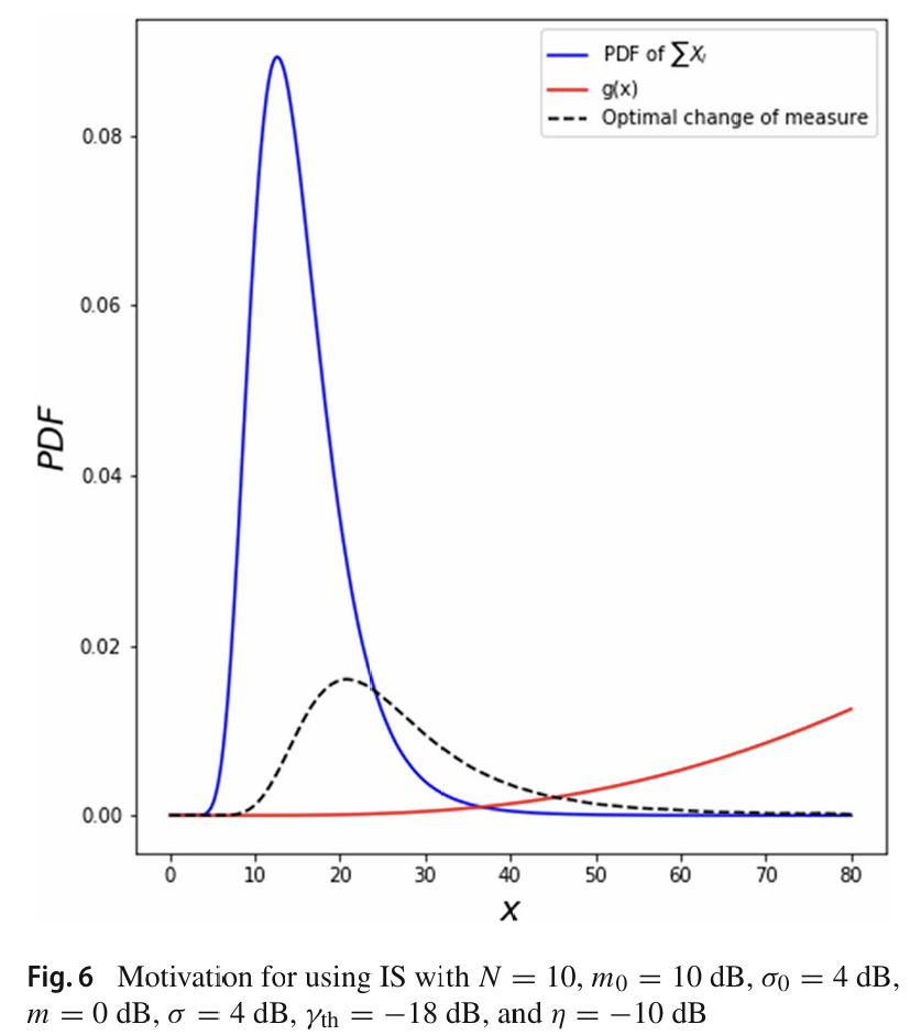
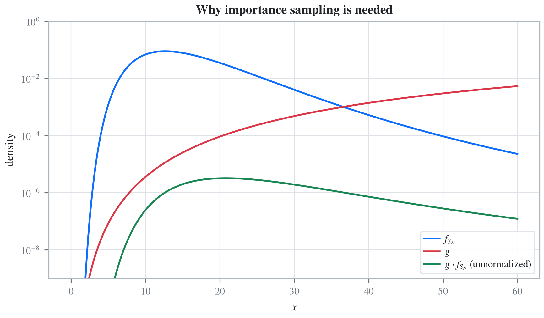
Figure 6, Figure 1, is the one figure in the paper that is not an efficiency metric. It plots the density of \(S_N\), the functional \(g\), and the unnormalized optimal importance sampling density \(g \cdot f_{S_N}\), to motivate why sampling from the original measure wastes effort. Figure 2 is the reproduction.
Figure 1: Ben Amar et al (2023), Figure 6.
import matplotlib.pyplot as pltgth = db(-18.0)g_vals = lognorm.cdf(gth * (xs + eta), shape0, scale=scale0)f_vals = density / S10b.bs # bucket mass to densityproduct = g_vals * f_valswindow = (xs >0) & (xs <60)fig, ax = plt.subplots(1, 1, figsize=(6.0, 3.5), layout='constrained')ax.plot(xs[window], f_vals[window], label=r'$f_{S_N}$')ax.plot(xs[window], g_vals[window], label=r'$g$')ax.plot(xs[window], product[window], label=r'$g \cdot f_{S_N}$(unnormalized)')ax.set_yscale('log')ax.set_ylim(1e-9, 1)ax.set_xlabel(r'$x$')ax.set_ylabel('density')ax.legend(loc='lower right', fontsize=8)ax.set_title('Why importance sampling is needed', fontsize=10)print(f'E[g(S)] = P_out(-18 dB) {product.sum() * S10b.bs:.6e}')print(f'mode of f_S {xs[np.argmax(f_vals)]:.4f}')print(f'mode of g . f_S {xs[np.argmax(product)]:.4f}')
E[g(S)] = P_out(-18 dB)   6.670881e-05
mode of f_S              12.6343
mode of g . f_S          20.8047
The rightward shift of the optimal sampling density is the whole point of Figure 1, and in Figure 2 it comes out at 12.63 against 20.80. Note that aggregate draws this figure with the exact \(f_{S_N}\), not with the moment-matched log-normal surrogate the paper’s own method has to fall back on.
7 Where the FFT method breaks down
The 4 dB target is \(2 \times 10^{-12}\), which is close to the floor of a double precision FFT. Table 4 shows how close.
rows = []for log2, bs in [(20, 2.0**-9), (21, 2.0**-10), (22, 2.0**-11), (23, 2.0**-12), (24, 2.0**-13)]: Sx = sum_of_lognormals(10, 0.0, 3.0, log2=log2, bs=bs) rows.append({'log2': log2, 'bs': f'2^{int(np.log2(bs))}','P(S_10 <= 2.51189)': Sx.cdf(db(4))})df = pd.DataFrame(rows)lo, hi = df['P(S_10 <= 2.51189)'].min(), df['P(S_10 <= 2.51189)'].max()print(f'spread across five grids: {(hi / lo -1) *100:.2f}%')GT(df)
spread across five grids: 1.09%
Table 4: The 4 dB probability across five grid settings, showing the spread the floor leaves behind.
log2
bs
P(S_10 <= 2.51189)
20
2^-9
2.358e-12
21
2^-10
2.343e-12
22
2^-11
2.336e-12
23
2^-12
2.332e-12
24
2^-13
2.334e-12
Two to three significant figures, and no more. The value is 2.33e-12 to 2.36e-12 across five grids spanning a factor of 16 in resolution. For a page like this that is a feature: it shows where the method’s floor actually is. The companion page on Ben Rached et al. (2024) quantifies that floor precisely, and it explains why it cannot be pushed lower by refining the grid.
8 Discussion
Ben Amar et al. (2023) is a variance reduction paper. Its contribution is an estimator, not a number, and the numbers exist only to establish that the regime is rare enough to be interesting. So the interesting comparison is not “does aggregate match their estimate” but “what does it cost to obtain the quantity at all”. Their best estimator needs a backward dynamic programming solve on a mesh of \(K = 20\) points for each of \(N\) steps, followed by \(M\) forward samples, and it delivers 5% relative error. The build above delivers the entire left tail curve, every threshold at once, to two or three significant figures, in a few seconds.
The second application is the sharper illustration. aggregate returns a density, and \(\mathsf E[g(S_N)]\) for any \(g\) is then a dot product against it. Changing \(g\) costs nothing. In the importance sampling framework, changing \(g\) changes the optimal control, so the entire backward solve has to be redone. That asymmetry, one distribution against one estimator per functional, is the argument.
The limits are obviously in the deep tail, where double precision FFT convolution runs out below roughly \(10^{-13}\), and any severity whose right tail is too heavy to carry on a uniform grid. Both are explored on the Ben Rached et al. (2024) page.
Programs in the aggregate Loss Lab
Each program below opens in the aggregate Loss Lab, which builds it with nothing to install. The names are those in reproductions.agg, where every program is renamed by its paper’s citation key.
BenAmar2023.S10: a sum of independent lognormals, the importance sampling test case.
BenAmar2023.S9: a sum of independent lognormals, the importance sampling test case.
Ben Amar, E., Ben Rached, N., Haji-Ali, A.-L., & Tempone, R. (2023). State-dependent importance sampling for estimating expectations of functionals of sums of independent random variables. Statistics and Computing. https://doi.org/10.1007/s11222-022-10202-2
Ben Rached, N., Hoel, H., & Meo, J. V. (2024). A fast and accurate numerical method for the left tail of sums of independent random variables. Statistics and Computing. https://doi.org/10.1007/s11222-024-10514-5