Asmussen, Jensen and Rojas-Nandayapa on the lognormal left tail

Reproducing Asmussen, Jensen and Rojas-Nandayapa (2016)

Author

Stephen J. Mildenhall

Published

2026-10-22 19:54 commit b5ca906+

1 The paper

Asmussen et al. (2016) studies the left tail of a sum of i.i.d. log-normals. The motivation is value at risk: if a portfolio of \(n\) assets has next-period values \(X_1, \dots, X_n\), each log-normal, then a loss corresponds to a small value of \(S_n = X_1 + \cdots + X_n\), and Basel II asks for quantiles as extreme as \(\alpha = 0.03\%\).

The distribution of a sum of \(n\) lognormals \(S_n\) is not available in explicit form and its numerical approximation is considered to be a challenging problem. In consequence, a number of methods for its evaluation has been developed across several decades, but these can rarely deliver arbitrary precisions in the whole support of the distribution, particularly in the tails.

The authors’ route is the Esscher transform. Because the right tail of the log-normal is heavy the moment generating function does not exist, but the Laplace transform \(L(\theta) = \mathsf E e^{-\theta X}\) is finite for all \(\theta \ge 0\), so the exponential family tilted toward the left is well defined. They obtain an asymptotic expression for \(L(\theta)\) in terms of the Lambert \(W\) function, approximate the Cramér function \(\theta(x)\) in closed form, and from these build two estimators: a saddlepoint approximation to \(F_n(nx)\) and \(f_n(nx)\), and an exponentially twisted importance sampling estimator.

This is exactly the sort of paper aggregate should be checked against, because unlike Ben Amar et al. (2023) it reports the actual quantities rather than the cost of estimating them.

2 What is reproducible

Fourteen tables are reproduced. Two of them, Table 1 (Newton-Raphson iterates for the saddlepoint) and Table 4 (powers of the Laplace transform), are internal to the authors’ algorithm and have no counterpart here. The other twelve are the CDF and PDF of \(S_n\) and are reproducible in full:

Table	Quantity	\(n\)	\(\sigma\)	Columns
2	CDF	4	0.250	Saddle0, Saddle1, two Monte Carlo variants
3	CDF	64	0.250	Saddle0, Saddle1
5	CDF	4	0.250	Saddle, MC with standard error
6	CDF	64	0.250	Saddle, MC with standard error
7	CDF	256	0.250	Saddle, MC with standard error
8	CDF	64	0.125	Saddle, MC with standard error
9	CDF	64	0.072	Saddle, MC with standard error
10 to 14	PDF	as above	as above	Saddle, MC with standard error

The parameter choices are stated:

A yearly volatility of order 0.25 is often argued to be typical. We have considered periods of lengths one year, one quarter, one month and one week, corresponding to \(\sigma = 0.25\), \(\sigma = 0.125\), \(\sigma = 0.072\), resp. \(\sigma = 0.035\). Real-life portfolios are often large, even in the thousands; the values we have chosen are \(n = 4, 16, 64, 256\). […] In all numerical experiments involving simulation we have employed \(R = 100{,}000\) replications.

Because the Monte Carlo columns carry standard errors, this is a reproduction with a built-in acceptance test: aggregate should sit within a standard error or two of the MC column.

3 Setup

Throughout, \(X \sim \mathrm{LN}(0, \sigma^2)\), so in scipy parameterization the scale is 1 and the shape is \(\sigma\). Sums are indexed so that every published table reports \(F_n(nx)\) and \(f_n(nx)\), that is, the argument is \(n\) times the tabulated \(x\).

%xmode minimal
import numpy as np
import pandas as pd
from functools import partial

from bookstyle import GT, build

# Tail probabilities and relative errors read as powers of ten, not SI prefixes.
GT = partial(GT, eng_style='exp')

def lognormal_sum(n, sigma, log2=22, bs=2.0 ** -12):
    """S_n = X_1 + ... + X_n with X_i iid LN(0, sigma^2).

    The count is deterministic, hence ``dfreq [n]``; the severity is written
    in scipy scale-shape form, ``sev 1 * lognorm sigma``.
    """
    return build(f'agg S dfreq [{n}] sev 1 * lognorm {sigma}',
                 log2=log2, bs=bs, normalize=False)

def compare(obj, rows, columns):
    """Assemble a comparison frame; ``rows`` are (x, n, paper values...)."""
    return pd.DataFrame([dict(zip(columns, r)) for r in rows])

Exception reporting mode: Minimal

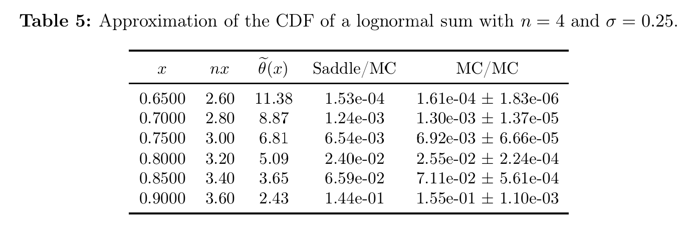
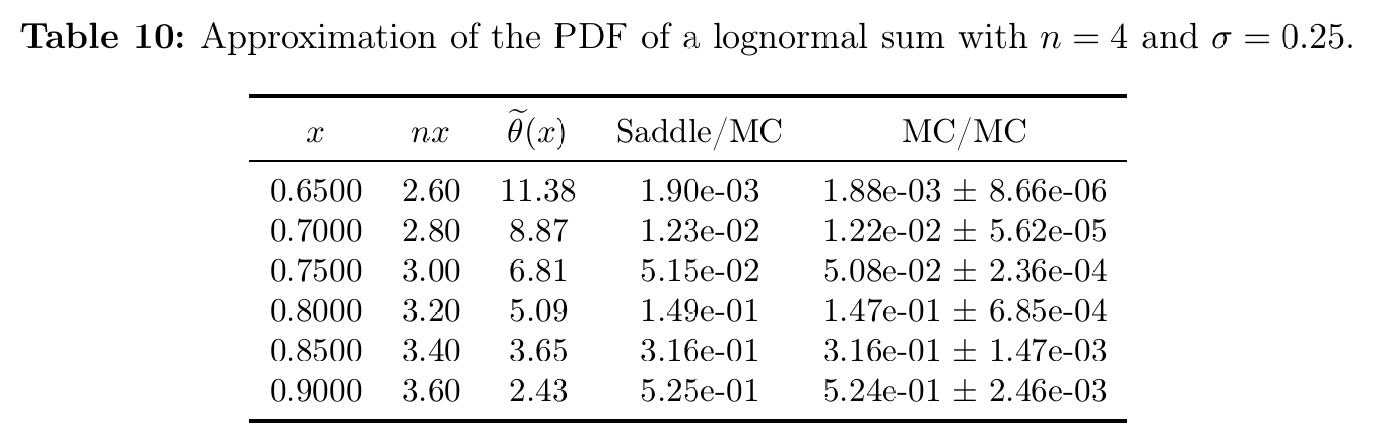
4 Tables 5 and 10: \(n = 4\), \(\sigma = 0.25\)

The smallest case, and the most demanding for a saddlepoint approximation, whose error is \(O(1/n)\) at first order. The targets are Figure 1 and Figure 2, reproduced in Table 1.

Figure 1: Asmussen, Jensen and Rojas-Nandayapa (2016), Table 5.

Figure 2: Asmussen, Jensen and Rojas-Nandayapa (2016), Table 10.

S4 = lognormal_sum(4, 0.25)

paper = [(0.65, 1.53e-4, 1.61e-4, 1.83e-6, 1.90e-3, 1.88e-3),
         (0.70, 1.24e-3, 1.30e-3, 1.37e-5, 1.23e-2, 1.22e-2),
         (0.75, 6.54e-3, 6.92e-3, 6.66e-5, 5.15e-2, 5.08e-2),
         (0.80, 2.40e-2, 2.55e-2, 2.24e-4, 1.49e-1, 1.47e-1),
         (0.85, 6.59e-2, 7.11e-2, 5.61e-4, 3.16e-1, 3.16e-1),
         (0.90, 1.44e-1, 1.55e-1, 1.10e-3, 5.25e-1, 5.24e-1)]

rows = []
for x, saddle, mc, se, saddle_pdf, mc_pdf in paper:
    nx = 4 * x
    cdf, pdf = S4.cdf(nx), S4.pdf(nx)
    rows.append({'x': x, 'nx': nx,
                 'Saddle CDF': saddle, 'MC CDF': mc, 'agg CDF': cdf,
                 'z': (cdf - mc) / se,
                 'Saddle PDF': saddle_pdf, 'MC PDF': mc_pdf, 'agg PDF': pdf})
GT(pd.DataFrame(rows))

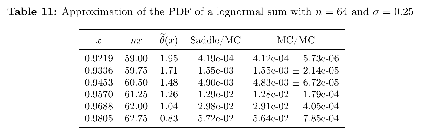
Table 1: Tables 5 and 10, \(n = 4\) at \(\sigma = 0.25\), the CDF and PDF against the saddlepoint and Monte Carlo columns.

x	nx	Saddle CDF	MC CDF	agg CDF	z	Saddle PDF	MC PDF	agg PDF
0.65000	2.600	0.00015	0.00016	0.00016	-1.03746	0.00190	0.00188	0.00187
0.70000	2.800	0.00124	0.00130	0.00130	-0.00791	0.01230	0.01220	0.01215
0.75000	3.000	0.00654	0.00692	0.00689	-0.51960	0.05150	0.05080	0.05077
0.80000	3.200	0.02400	0.02550	0.02552	0.07434	0.14900	0.14700	0.14734
0.85000	3.400	0.06590	0.07110	0.07071	-0.69297	0.31600	0.31600	0.31553
0.90000	3.600	0.14400	0.15500	0.15444	-0.50661	0.52500	0.52400	0.52328

Every agg value sits within about one Monte Carlo standard error of the MC column. The saddlepoint column is systematically 4% to 7% low, which is the expected \(O(1/n)\) behavior at \(n = 4\).

5 Table 3: `aggregate` as referee between first and second order

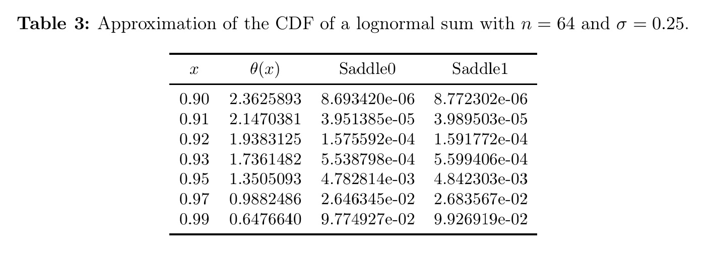
Table 3, Figure 3, is the interesting one, because it reports the first-order and second-order saddlepoint side by side with no Monte Carlo column to arbitrate between them.

General results for the saddlepoint approximation state that for a fixed \(x\) the relative error is \(O(1/n)\) for the first order approximation and \(O(1/n^2)\) for the second order approximation.

aggregate supplies the missing reference value.

Figure 3: Asmussen, Jensen and Rojas-Nandayapa (2016), Table 3.

S64 = lognormal_sum(64, 0.25)

paper = [(0.90, 8.693420e-06, 8.772302e-06),
         (0.91, 3.951385e-05, 3.989503e-05),
         (0.92, 1.575592e-04, 1.591772e-04),
         (0.93, 5.538798e-04, 5.599406e-04),
         (0.95, 4.782814e-03, 4.842303e-03),
         (0.97, 2.646345e-02, 2.683567e-02),
         (0.99, 9.774927e-02, 9.926919e-02)]

rows = []
for x, s0, s1 in paper:
    ref = S64.cdf(64 * x)
    rows.append({'x': x, 'nx': 64 * x, 'Saddle0': s0, 'Saddle1': s1,
                 'agg': ref,
                 'Saddle0 rel err': s0 / ref - 1,
                 'Saddle1 rel err': s1 / ref - 1})
GT(pd.DataFrame(rows))

Table 2: Table 3, the first and second order saddlepoint at \(n = 64\), with the library supplying the missing reference column.

x	nx	Saddle0	Saddle1	agg	Saddle0 rel err	Saddle1 rel err
0.90000	57.60	8.693e-06	8.772e-06	8.771e-06	-8.87e-03	1.22e-04
0.91000	58.24	39.514e-06	39.895e-06	39.903e-06	-9.75e-03	-1.93e-04
0.92000	58.88	157.559e-06	159.177e-06	159.169e-06	-1.01e-02	4.97e-05
0.93000	59.52	553.880e-06	559.941e-06	559.801e-06	-1.06e-02	2.50e-04
0.95000	60.80	4.783e-03	4.842e-03	4.842e-03	-1.21e-02	1.64e-04
0.97000	62.08	26.463e-03	26.836e-03	26.833e-03	-1.38e-02	9.77e-05
0.99000	63.36	97.749e-03	99.269e-03	99.264e-03	-1.53e-02	4.97e-05

Table 2 is unambiguous. At \(n = 64\) the first-order saddlepoint runs from 0.9% to 1.5% low across the range, and the second-order saddlepoint is correct to within three parts in \(10^4\) everywhere. The second-order correction buys roughly two orders of magnitude, and aggregate can say so because it is not itself a saddlepoint method.

A cleaner comparison is available because Tables 2 and 3 share the point \(x = 0.90\) at \(\sigma = 0.25\), differing only in \(n\), and Table 3 makes it.

shared = [(4, 3.6, 0.1456850237, 0.1545557418, S4),
          (64, 57.6, 8.693420e-06, 8.772302e-06, S64)]
rows = []
for n, nx, s0, s1, obj in shared:
    ref = obj.cdf(nx)
    rows.append({'n': n, 'x': 0.90, 'agg': ref,
                 'Saddle0 rel err': s0 / ref - 1,
                 'Saddle1 rel err': s1 / ref - 1})
GT(pd.DataFrame(rows))

Table 3: The two saddlepoint orders at the one abscissa Tables 2 and 3 share, at \(n = 4\) and \(n = 64\).

n	x	agg	Saddle0 rel err	Saddle1 rel err
4	0.90000	154.443e-03	-5.67e-02	7.32e-04
64	0.90000	8.771e-06	-8.87e-03	1.22e-04

In Table 3 both orders improve by a factor of roughly six going from \(n = 4\) to \(n = 64\). That is far short of the 16 and 256 that the stated \(O(1/n)\) and \(O(1/n^2)\) rates would suggest, but the comparison is not the one those rates describe: holding \(x = 0.90\) fixed while raising \(n\) drives the probability from 0.154 down to \(8.8 \times 10^{-6}\), so the two rows are not in the same regime. Read it as a measurement, not as a rate test.

6 Tables 6 and 11: \(n = 64\), \(\sigma = 0.25\)

The targets are Figure 4 and Figure 5, reproduced in Table 4.

Figure 4: Asmussen, Jensen and Rojas-Nandayapa (2016), Table 6.

Figure 5: Asmussen, Jensen and Rojas-Nandayapa (2016), Table 11.

paper = [(0.9219, 59.00, 2.00e-4, 2.04e-4, 2.56e-6, 4.19e-4, 4.12e-4),
         (0.9336, 59.75, 8.31e-4, 8.56e-4, 1.01e-5, 1.55e-3, 1.55e-3),
         (0.9453, 60.50, 2.97e-3, 3.06e-3, 3.35e-5, 4.90e-3, 4.83e-3),
         (0.9570, 61.25, 8.99e-3, 9.22e-3, 9.43e-5, 1.29e-2, 1.28e-2),
         (0.9688, 62.00, 2.40e-2, 2.45e-2, 2.30e-4, 2.98e-2, 2.91e-2),
         (0.9805, 62.75, 5.45e-2, 5.59e-2, 4.79e-4, 5.72e-2, 5.64e-2)]

rows = []
for x, nx, saddle, mc, se, saddle_pdf, mc_pdf in paper:
    cdf, pdf = S64.cdf(nx), S64.pdf(nx)
    rows.append({'x': x, 'nx': nx, 'Saddle CDF': saddle, 'MC CDF': mc,
                 'agg CDF': cdf, 'z': (cdf - mc) / se,
                 'Saddle PDF': saddle_pdf, 'MC PDF': mc_pdf, 'agg PDF': pdf})
GT(pd.DataFrame(rows))

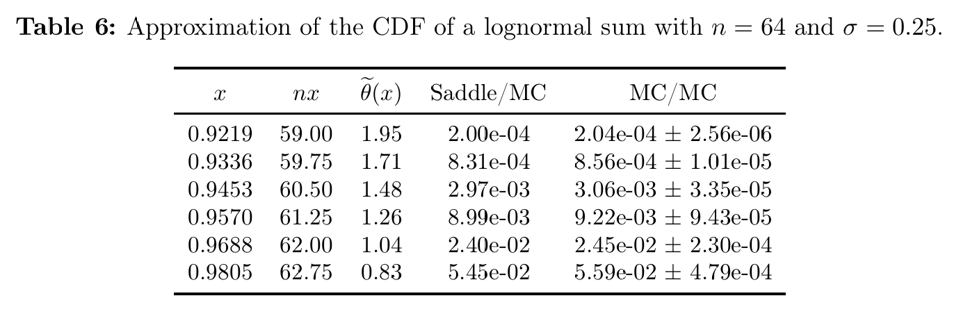
Table 4: Tables 6 and 11, \(n = 64\) at \(\sigma = 0.25\), the CDF and PDF against the saddlepoint and Monte Carlo columns.

x	nx	Saddle CDF	MC CDF	agg CDF	z	Saddle PDF	MC PDF	agg PDF
0.92190	59.00	0.00020	0.00020	0.00020	-0.20914	0.00042	0.00041	0.00041
0.93360	59.75	0.00083	0.00086	0.00085	-0.17581	0.00155	0.00155	0.00154
0.94530	60.50	0.00297	0.00306	0.00304	-0.46655	0.00490	0.00483	0.00484
0.95700	61.25	0.00899	0.00922	0.00928	0.66760	0.01290	0.01280	0.01286
0.96880	62.00	0.02400	0.02450	0.02441	-0.38119	0.02980	0.02910	0.02915
0.98050	62.75	0.05450	0.05590	0.05583	-0.15317	0.05720	0.05640	0.05657

7 Tables 7 and 12: \(n = 256\), \(\sigma = 0.25\)

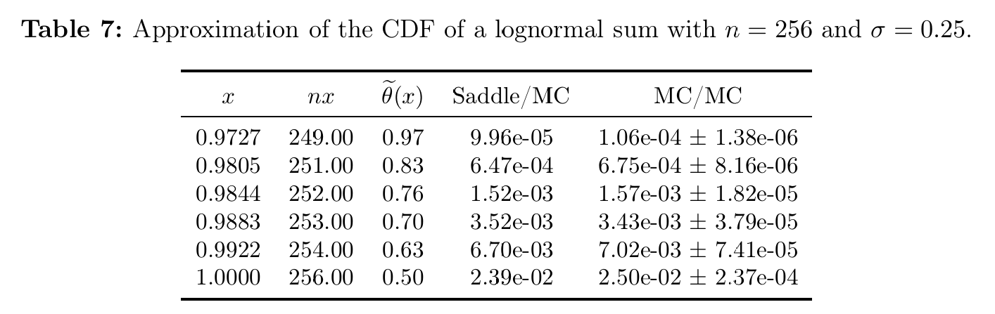
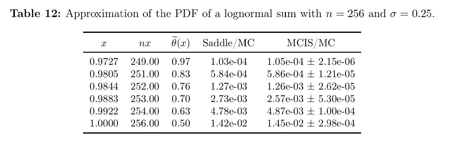
A 256-fold convolution, which is the case the authors describe as realistic for a large portfolio. It costs the same single build. The targets are Figure 6 and Figure 7, reproduced in Table 5.

Figure 6: Asmussen, Jensen and Rojas-Nandayapa (2016), Table 7.

Figure 7: Asmussen, Jensen and Rojas-Nandayapa (2016), Table 12.

S256 = lognormal_sum(256, 0.25)

paper = [(0.9727, 249.0, 9.96e-5, 1.06e-4, 1.38e-6, 1.03e-4, 1.05e-4),
         (0.9805, 251.0, 6.47e-4, 6.75e-4, 8.16e-6, 5.84e-4, 5.86e-4),
         (0.9844, 252.0, 1.52e-3, 1.57e-3, 1.82e-5, 1.27e-3, 1.26e-3),
         (0.9883, 253.0, 3.52e-3, 3.43e-3, 3.79e-5, 2.73e-3, 2.57e-3),
         (0.9922, 254.0, 6.70e-3, 7.02e-3, 7.41e-5, 4.78e-3, 4.87e-3),
         (1.0000, 256.0, 2.39e-2, 2.50e-2, 2.37e-4, 1.42e-2, 1.45e-2)]

rows = []
for x, nx, saddle, mc, se, saddle_pdf, mc_pdf in paper:
    cdf, pdf = S256.cdf(nx), S256.pdf(nx)
    rows.append({'x': x, 'nx': nx, 'Saddle CDF': saddle, 'MC CDF': mc,
                 'agg CDF': cdf, 'z': (cdf - mc) / se,
                 'Saddle PDF': saddle_pdf, 'MC PDF': mc_pdf, 'agg PDF': pdf})
GT(pd.DataFrame(rows))

Table 5: Tables 7 and 12, \(n = 256\) at \(\sigma = 0.25\), the CDF and PDF against the saddlepoint and Monte Carlo columns.

x	nx	Saddle CDF	MC CDF	agg CDF	z	Saddle PDF	MC PDF	agg PDF
0.97270	249	0.00010	0.00011	0.00010	-1.69690	0.00010	0.00011	0.00010
0.98050	251	0.00065	0.00068	0.00067	-0.05182	0.00058	0.00059	0.00059
0.98440	252	0.00152	0.00157	0.00157	-0.23734	0.00127	0.00126	0.00127
0.98830	253	0.00352	0.00343	0.00342	-0.32962	0.00273	0.00257	0.00256
0.99220	254	0.00670	0.00702	0.00702	0.05763	0.00478	0.00487	0.00485
1.00000	256	0.02390	0.02500	0.02491	-0.37478	0.01420	0.01450	0.01435

7.1 A probable error in the published table

The \(x = 0.9883\) row of Table 5 deserves attention. Everywhere else in Tables 7 and 12 the saddlepoint value sits below the Monte Carlo value, by 3% to 5% for the CDF and by 0% to 1.5% for the PDF, which is the systematic bias expected of the approximation. At \(x = 0.9883\) both entries jump the other way: the CDF is 3.0% above the reference and the PDF is 6.5% above, as Table 6 isolates.

paper = [(0.9727, 249.0, 9.96e-5, 1.06e-4, 1.03e-4, 1.05e-4),
         (0.9805, 251.0, 6.47e-4, 6.75e-4, 5.84e-4, 5.86e-4),
         (0.9844, 252.0, 1.52e-3, 1.57e-3, 1.27e-3, 1.26e-3),
         (0.9883, 253.0, 3.52e-3, 3.43e-3, 2.73e-3, 2.57e-3),
         (0.9922, 254.0, 6.70e-3, 7.02e-3, 4.78e-3, 4.87e-3),
         (1.0000, 256.0, 2.39e-2, 2.50e-2, 1.42e-2, 1.45e-2)]

rows = []
for x, nx, saddle, mc, saddle_pdf, mc_pdf in paper:
    cdf, pdf = S256.cdf(nx), S256.pdf(nx)
    rows.append({'x': x,
                 'Saddle CDF vs agg': saddle / cdf - 1,
                 'MC CDF vs agg': mc / cdf - 1,
                 'Saddle PDF vs agg': saddle_pdf / pdf - 1,
                 'MC PDF vs agg': mc_pdf / pdf - 1})
GT(pd.DataFrame(rows))

Table 6: Each published column as a relative difference from the library, showing the sign flip at one abscissa.

x	Saddle CDF vs agg	MC CDF vs agg	Saddle PDF vs agg	MC PDF vs agg
0.97270	-0.03915	0.02259	-0.00689	0.01240
0.98050	-0.04088	0.00063	-0.00834	-0.00495
0.98440	-0.02918	0.00276	0.00017	-0.00771
0.98830	0.02999	0.00366	0.06475	0.00235
0.99220	-0.04616	-0.00061	-0.01489	0.00366
1.00000	-0.04059	0.00357	-0.01046	0.01044

In Table 6 the Monte Carlo columns agree with aggregate at every row, including \(x = 0.9883\), where the CDF is within 0.33 standard errors and the PDF within 0.11. Only the two saddlepoint entries are out of line, and they are out of line together. A single mis-solved \(\theta(x)\) at that one abscissa would produce exactly this pattern, since both the CDF and the PDF saddlepoint formulas take \(\theta(x)\) as input. The evidence points to an error in that row of the published tables rather than to a failure of the method, but it is worth flagging rather than quietly averaging over.

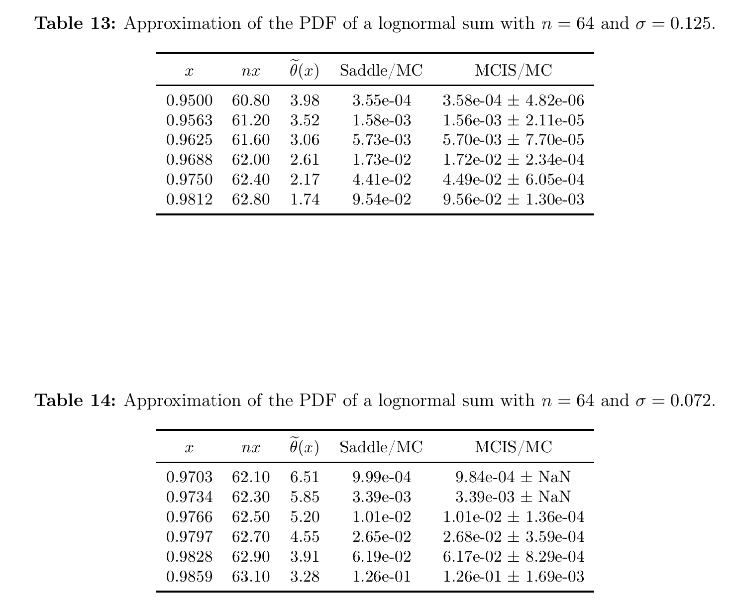
8 Tables 8, 9, 13 and 14: shorter horizons

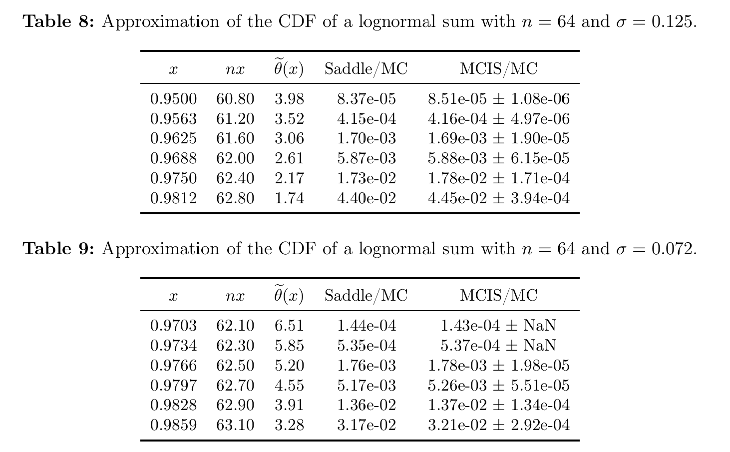
Quarterly and monthly volatility, \(n = 64\). The targets are Figure 8 and Figure 9, reproduced in Table 7.

Figure 8: Asmussen, Jensen and Rojas-Nandayapa (2016), Tables 8 and 9.

Figure 9: Asmussen, Jensen and Rojas-Nandayapa (2016), Tables 13 and 14.

cases = {
    0.125: [(0.9500, 60.80, 8.37e-5, 8.51e-5, 3.55e-4, 3.58e-4),
            (0.9563, 61.20, 4.15e-4, 4.16e-4, 1.58e-3, 1.56e-3),
            (0.9625, 61.60, 1.70e-3, 1.69e-3, 5.73e-3, 5.70e-3),
            (0.9688, 62.00, 5.87e-3, 5.88e-3, 1.73e-2, 1.72e-2),
            (0.9750, 62.40, 1.73e-2, 1.78e-2, 4.41e-2, 4.49e-2),
            (0.9812, 62.80, 4.40e-2, 4.45e-2, 9.54e-2, 9.56e-2)],
    0.072: [(0.9703, 62.10, 1.44e-4, 1.43e-4, 9.99e-4, 9.84e-4),
            (0.9734, 62.30, 5.35e-4, 5.37e-4, 3.39e-3, 3.39e-3),
            (0.9766, 62.50, 1.76e-3, 1.78e-3, 1.01e-2, 1.01e-2),
            (0.9797, 62.70, 5.17e-3, 5.26e-3, 2.65e-2, 2.68e-2),
            (0.9828, 62.90, 1.36e-2, 1.37e-2, 6.19e-2, 6.17e-2),
            (0.9859, 63.10, 3.17e-2, 3.21e-2, 1.26e-1, 1.26e-1)],
}

frames = []
for sigma, paper in cases.items():
    obj = lognormal_sum(64, sigma)
    for x, nx, saddle, mc, saddle_pdf, mc_pdf in paper:
        frames.append({'sigma': sigma, 'x': x, 'nx': nx,
                       'Saddle CDF': saddle, 'MC CDF': mc,
                       'agg CDF': obj.cdf(nx),
                       'Saddle PDF': saddle_pdf, 'MC PDF': mc_pdf,
                       'agg PDF': obj.pdf(nx)})
GT(pd.DataFrame(frames))

Table 7: Tables 8, 9, 13 and 14, quarterly and monthly volatility at \(n = 64\), against the saddlepoint and Monte Carlo columns.

sigma	x	nx	Saddle CDF	MC CDF	agg CDF	Saddle PDF	MC PDF	agg PDF
0.12500	0.95000	60.80	0.00008	0.00009	0.00008	0.00036	0.00036	0.00035
0.12500	0.95630	61.20	0.00042	0.00042	0.00041	0.00158	0.00156	0.00156
0.12500	0.96250	61.60	0.00170	0.00169	0.00171	0.00573	0.00570	0.00569
0.12500	0.96880	62.00	0.00587	0.00588	0.00596	0.01730	0.01720	0.01738
0.12500	0.97500	62.40	0.01730	0.01780	0.01767	0.04410	0.04490	0.04452
0.12500	0.98120	62.80	0.04400	0.04450	0.04484	0.09540	0.09560	0.09597
0.07200	0.97030	62.10	0.00014	0.00014	0.00014	0.00100	0.00098	0.00099
0.07200	0.97340	62.30	0.00053	0.00054	0.00054	0.00339	0.00339	0.00338
0.07200	0.97660	62.50	0.00176	0.00178	0.00178	0.01010	0.01010	0.01012
0.07200	0.97970	62.70	0.00517	0.00526	0.00523	0.02650	0.02680	0.02662
0.07200	0.98280	62.90	0.01360	0.01370	0.01366	0.06190	0.06170	0.06163
0.07200	0.98590	63.10	0.03170	0.03210	0.03181	0.12600	0.12600	0.12563

At \(\sigma = 0.072\) the summands are nearly deterministic and all three methods coincide to three figures. The interest is at \(\sigma = 0.25\), where they separate.

9 Discussion

Twelve tables, both CDF and PDF, \(n\) from 4 to 256, \(\sigma\) from 0.072 to 0.25, all reproduced from five build calls. aggregate sits inside the Monte Carlo error bars throughout, which is the acceptance test the paper itself supplies.

The more useful outcome is the referee role. The paper reports two saddlepoint orders and a Monte Carlo estimate with 100,000 replications, and in several places they disagree at the third significant figure. Because aggregate is neither a saddlepoint expansion nor a sampler, it can adjudicate: the second-order saddlepoint is accurate to a few parts in \(10^4\) at \(n = 64\), the first-order version is about 1% low, and where the two published columns conflict at \(n = 256\) the Monte Carlo column is the one to trust.

None of this diminishes the paper. The saddlepoint approximation costs almost nothing to evaluate once the Lambert \(W\) machinery is in place, and it extends to regimes far beyond what any grid method can reach. The reproduction below \(10^{-13}\) is not attempted here for exactly that reason, and the companion page on Ben Rached et al. (2024) explains where the FFT floor sits and why refining the grid does not move it.

The parameterization is worth recording, since it is the one place a reproduction can silently go wrong. The paper writes \(X \sim \mathrm{LN}(0, \sigma^2)\) with \(\mu = 0\) throughout, noting that \(\mu\) is only a scaling factor, and tabulates against \(x\) while evaluating at \(nx\). In DecL that is sev 1 * lognorm sigma with dfreq [n], and the argument to cdf is \(n x\).

Programs in the aggregate Loss Lab

Each program below opens in the aggregate Loss Lab, which builds it with nothing to install. The names are those in reproductions.agg, where every program is renamed by its paper’s citation key.

Asmussen2016a.S: a sum of independent lognormals, the saddlepoint test case.
Asmussen2016a.S.v2: a sum of independent lognormals, the saddlepoint test case.

Asmussen, S., Jensen, J. L., & Rojas-Nandayapa, L. (2016). Exponential Family Techniques for the Lognormal Left Tail. Scandinavian Journal of Statistics, 43(3), 774–787. https://doi.org/10.1111/sjos.12203

Ben Amar, E., Ben Rached, N., Haji-Ali, A.-L., & Tempone, R. (2023). State-dependent importance sampling for estimating expectations of functionals of sums of independent random variables. Statistics and Computing. https://doi.org/10.1007/s11222-022-10202-2

Ben Rached, N., Hoel, H., & Meo, J. V. (2024). A fast and accurate numerical method for the left tail of sums of independent random variables. Statistics and Computing. https://doi.org/10.1007/s11222-024-10514-5