Wang and risk loads by layer

Reproducing Wang (2000), Table 1

Author

Stephen J. Mildenhall

Published

2026-10-22 19:56 commit b5ca906+

1 Context and problem

Wang (2000) introduces the distortion operator now known as the Wang transform,

\[g_\alpha(u) = \Phi\!\left(\Phi^{-1}(u) + \alpha\right),\]

and argues for it against the proportional hazard transform of Wang (1995), $g_r(u) = u^{r}$, which had been the actuarial default for pricing by layer. Both are distortions, so both price a layer by integrating the distorted survival function over it, and both give a risk load that grows with the layer. The paper’s case is about how fast.

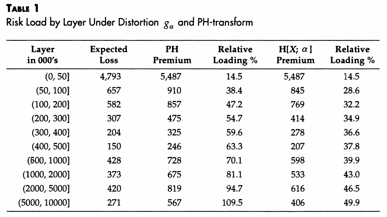
The criterion comes from Venter (1991): market prices by layer imply a distortion, and the distortion has to produce a relative loading that increases with the layer, since that is what observed reinsurance prices do. The PH transform does that. The paper’s complaint is that it does it too fast at high layers, and Table 1 is the demonstration.

This is a reproduction of a pricing exhibit rather than a numerical method, so what is being tested is aggregate’s distortion machinery and its layer decomposition: lev for the expected loss and exag for the distorted equivalent, differenced across a tower.

2 Paper solution and gold standard

Example 1 takes a ground-up liability risk with a Pareto survival function

\[S_X(x) = \left(\frac{2000}{2000 + x}\right)^{1.2}, \qquad x > 0,\]

which is a Lomax with shape 1.2 and scale 2000, and assumes exactly one claim. The Wang loading is $\alpha = 0.1$. The PH index is then chosen as $r = 0.9245$ “to yield the same relative loading (14.5 percent) for the basic limit layer $(\$0, \$50{,}000]$”, which makes the first row a calibration rather than a result.

Table 1, Figure 1, gives, for ten layers, the expected loss, the PH premium and loading, and the Wang premium and loading. Table 1 transcribes it.

%xmode minimal
import numpy as np
import pandas as pd
from bookstyle import GT, build, show

ALPHA, THETA = 1.2, 2000.0
LAYERS = [0, 50e3, 100e3, 200e3, 300e3, 400e3, 500e3, 1000e3, 2000e3, 5000e3, 10000e3]
NAMES = [f'({int(a/1000)}, {int(b/1000)}]' for a, b in zip(LAYERS[:-1], LAYERS[1:])]
PAPER = pd.DataFrame(
    {'expected loss': [4793, 657, 582, 307, 204, 150, 428, 373, 420, 271],
     'PH premium': [5487, 910, 857, 475, 325, 246, 728, 675, 819, 567],
     'PH loading %': [14.5, 38.4, 47.2, 54.7, 59.6, 63.3, 70.1, 81.1, 94.7, 109.5],
     'Wang premium': [5487, 845, 769, 414, 278, 207, 598, 533, 616, 406],
     'Wang loading %': [14.5, 28.6, 32.2, 34.9, 36.6, 37.8, 39.9, 43.0, 46.5, 49.9]},
    index=NAMES)
GT(PAPER, float_format=1)

Exception reporting mode: Minimal

Table 1: Wang (2000), Table 1 as printed.

level_0	expected loss	PH premium	PH loading %	Wang premium	Wang loading %
(0, 50]	4,793	5,487	14.5	5,487	14.5
(50, 100]	657	910	38.4	845	28.6
(100, 200]	582	857	47.2	769	32.2
(200, 300]	307	475	54.7	414	34.9
(300, 400]	204	325	59.6	278	36.6
(400, 500]	150	246	63.3	207	37.8
(500, 1000]	428	728	70.1	598	39.9
(1000, 2000]	373	675	81.1	533	43.0
(2000, 5000]	420	819	94.7	616	46.5
(5000, 10000]	271	567	109.5	406	49.9

The expected loss column has a closed form, which is what makes Table 1 worth checking rather than merely reproducing. A Lomax has

\[\mathsf E[X \wedge a] = \frac{\theta}{\alpha - 1}\left(1 - \left(\frac{\theta}{\theta + a}\right)^{\alpha - 1}\right),\]

so every layer expected loss is a difference of two elementary expressions, checked in Table 2.

def lev(a):
    return THETA / (ALPHA - 1) * (1 - (THETA / (THETA + a)) ** (ALPHA - 1))

cl = np.diff([lev(a) for a in LAYERS])
chk = pd.DataFrame({'closed form': cl, 'Table 1': PAPER['expected loss'].to_numpy()},
                   index=NAMES)
chk['difference'] = chk['closed form'] - chk['Table 1']
chk['rounding explains it'] = chk['difference'].abs() < 0.5
GT(chk, formatters={'closed form': 2, 'Table 1': 0,
                    # GT format sugar has no sign flag, so the signed column
                    # goes through a callable; `formatters` takes one, and
                    # `float_format` deliberately does not.
                    'difference': lambda x: f'{x:+.2f}'})

Table 2: The ten layer expected losses in closed form, against the column Table 1 prints.

level_0	closed form	Table 1	difference	rounding explains it
(0, 50]	4,787.99	4,793	-5.01	False
(50, 100]	657.04	657	+0.04	True
(100, 200]	581.82	582	-0.18	True
(200, 300]	307.05	307	+0.05	True
(300, 400]	203.83	204	-0.17	True
(400, 500]	150.46	150	+0.46	True
(500, 1000]	427.56	428	-0.44	True
(1000, 2000]	372.86	373	-0.14	True
(2000, 5000]	420.27	420	+0.27	True
(5000, 10000]	270.62	271	-0.38	True

In Table 2, nine of the ten layers agree with the closed form to within half a dollar, which is exactly what rounding to the nearest dollar allows. The basic limit layer does not: the closed form gives 4,787.99 and the paper prints 4,793, a difference of 5.01. That cannot be rounding, and it is the same row the technical guides flagged as looking wrong without pinning it down.

3 The `aggregate` reproduction

The tower goes in as an occurrence cession, and the distortions as their own objects. Table 3 confirms the grid before any pricing is read off it.

a1 = build('agg Wang.Layers 1 claim 10000e3 xs 0 sev 2000 * lomax 1.2 '
           f'occurrence ceded to tower {LAYERS} fixed', bs=20, log2=20)
show(a1)
d_wang = build(f'distortion wang_a wang 0.1')
d_ph = build(f'distortion ph_r ph 0.9245')
show(d_wang)
show(d_ph)

agg Wang.Layers
  1 claim
  10000000 xs 0
  sev 2000 * lomax 1.2
  occurrence ceded to
    50000 xs 0 and
    50000 xs 50000 and
    100000 xs 100000 and
    100000 xs 200000 and
    100000 xs 300000 and
    100000 xs 400000 and
    500000 xs 500000 and
    1000000 xs 1000000 and
    3000000 xs 2000000 and
    5000000 xs 5000000
  fixed

distortion wang_a wang 0.1

distortion ph_r ph 0.9245

GT(pd.DataFrame([
    {'quantity': 'E[X and 10M], aggregate', 'value': a1.est_m},
    {'quantity': 'E[X and 10M], closed form', 'value': lev(10e6)},
    {'quantity': 'relative difference',
     'value': abs(a1.est_m / lev(10e6) - 1)},
]).set_index('quantity'), formatters={'value': '{x:.6g}'})

Table 3: The limited expected value at the top of the tower, against the closed form.

quantity	value
E[X and 10M], aggregate	8179.5
E[X and 10M], closed form	8179.51
relative difference	1.22254e-06

def by_layer(dist):
    a1.apply_distortion(dist)
    d = a1.density_df.loc[LAYERS, ['lev', 'exag']]
    return np.diff(d.lev.to_numpy()), np.diff(d.exag.to_numpy())

el_w, pr_w = by_layer(d_wang)
el_p, pr_p = by_layer(d_ph)
got = pd.DataFrame({'expected loss': el_w, 'PH premium': pr_p,
                    'PH loading %': 100 * (pr_p / el_p - 1),
                    'Wang premium': pr_w,
                    'Wang loading %': 100 * (pr_w / el_w - 1)}, index=NAMES)
GT(pd.concat({'paper': PAPER, 'aggregate': got}, axis=1), float_format=1)

Table 4: Table 1 rebuilt, all five columns over the ten layer tower, beside the printed figures.

	paper					aggregate
level_0	expected loss	PH premium	PH loading %	Wang premium	Wang loading %	expected loss	PH premium	PH loading %	Wang premium	Wang loading %
(0, 50]	4,793	5,487	14.5	5,487	14.5	4,788.0	5,481.4	14.5	5,481.8	14.5
(50, 100]	657	910	38.4	845	28.6	657.0	909.5	38.4	845.0	28.6
(100, 200]	582	857	47.2	769	32.2	581.8	856.4	47.2	768.9	32.2
(200, 300]	307	475	54.7	414	34.9	307.1	474.9	54.7	414.2	34.9
(300, 400]	204	325	59.6	278	36.6	203.8	325.3	59.6	278.4	36.6
(400, 500]	150	246	63.3	207	37.8	150.5	245.7	63.3	207.3	37.8
(500, 1000]	428	728	70.1	598	39.9	427.6	727.4	70.1	598.0	39.9
(1000, 2000]	373	675	81.1	533	43.0	372.9	675.3	81.1	533.2	43.0
(2000, 5000]	420	819	94.7	616	46.5	420.3	818.4	94.7	615.6	46.5
(5000, 10000]	271	567	109.5	406	49.9	270.6	567.0	109.5	405.7	49.9

rel = (got / PAPER - 1).abs()
GT(pd.DataFrame([
    {'column': c, 'worst relative difference': float(rel[c].max()),
     'worst layer': rel[c].idxmax()} for c in PAPER.columns]
    + [{'column': 'all fifty', 'worst relative difference': float(rel.max().max()),
        'worst layer': ''}]).set_index('column'),
   formatters={'worst relative difference': '{x:.2e}'})

Table 5: Worst relative difference from the printed table, column by column and over all fifty entries.

column	worst relative difference	worst layer
expected loss	3.07e-03	(400, 500]
PH premium	1.15e-03	(400, 500]
PH loading %	1.22e-03	(0, 50]
Wang premium	1.48e-03	(400, 500]
Wang loading %	1.16e-03	(100, 200]
all fifty	3.07e-03

Table 4 and Table 5 have all fifty published entries reproducing to within 0.31% relative, and every loading percentage matching to the tenth of a point printed. The paper’s qualitative claim is the one it cares about and it comes back clearly: the PH loading runs from 14.5% to 109.5% across the tower while the Wang loading runs from 14.5% to 49.9%, so at the top layer the PH transform is charging more than twice the relative load for the same risk.

4 Comments

4.1 The basic limit entry is misprinted, and the loading column proves it

Two independent arguments say the 4,793 is wrong and 4,788 is right.

The closed form gives 4,787.99, and the other nine layers all agree with the closed form to within rounding, so the method of computing the column was sound everywhere else.

And the paper’s own construction pins the row. The PH index $r = 0.9245$ was chosen to give the same 14.5% loading on this layer as the Wang transform does, and both premium columns print 5,487 for it. Table 6 checks what loading 5,487 implies against each candidate expected loss.

for_el = [4787.99, 4793]
GT(pd.DataFrame([
    {'expected loss used': e,
     'implied loading from a premium of 5487 %': 100 * (5487 / e - 1),
     'paper prints': 14.5} for e in for_el]).set_index('expected loss used'),
   float_format=3)

Table 6: The loading a premium of 5,487 implies against each candidate basic limit expected loss.

expected loss used	implied loading from a premium of 5487 %	paper prints
4,787.990	14.599	14.500
4,793.000	14.479	14.500

In Table 6, against 4,788 a premium of 5,487 is a 14.6% loading; against 4,793 it is 14.5%. So the printed premium and the printed loading are consistent with each other and with 4,793, which says the error is upstream of the table: the expected loss was computed as 4,793 and then everything in the row was derived from it. It is a single wrong input, not a typo in one cell.

Nothing downstream depends on it. The row is a calibration, so its only job is to fix $r$, and by Table 7 $r$ would move in the fourth decimal.

from scipy.optimize import brentq

def ph_loading(r):
    d = build(f'distortion tmp ph {r}')
    a1.apply_distortion(d)
    dd = a1.density_df.loc[[0, 50e3], ['lev', 'exag']]
    el = dd.lev.iloc[1] - dd.lev.iloc[0]
    pr = dd.exag.iloc[1] - dd.exag.iloc[0]
    return pr / el - 1

r_star = brentq(lambda r: ph_loading(r) - (5487 / 4787.99 - 1), 0.90, 0.95,
                xtol=1e-7)
GT(pd.DataFrame([
    {'quantity': "paper's PH index", 'value': 0.9245},
    {'quantity': 'index matching the closed-form loading', 'value': r_star},
    {'quantity': 'difference', 'value': r_star - 0.9245},
]).set_index('quantity'), float_format=7)

Table 7: The PH index recalibrated against the closed form basic limit loss, beside the paper’s.

quantity	value
paper's PH index	0.9245000
index matching the closed-form loading	0.9239451
difference	-0.0005549

4.2 The tower is a cession, not ten builds

Worth noting how little code Table 4 needs. occurrence ceded to tower [...] declares all ten layers in one clause, and the layer expected losses and distorted premiums are then differences of two density_df columns, lev and exag, read at the layer boundaries. There is no loop over layers and no per-layer object.

That works because a distortion price is an integral of the distorted survival function, so it is additive across layers in exactly the way the expected loss is. That additivity is the mathematical content of Venter (1991)’s observation and the reason a distortion is the right object for layer pricing in the first place: a risk measure without it would not let a tower be priced consistently layer by layer.

4.3 Where the two transforms actually differ

Table 8 puts the two loading columns side by side with their ratio.

GT(pd.DataFrame([
    {'layer': n, 'PH loading %': got.loc[n, 'PH loading %'],
     'Wang loading %': got.loc[n, 'Wang loading %'],
     'ratio': got.loc[n, 'PH loading %'] / got.loc[n, 'Wang loading %']}
    for n in NAMES]).set_index('layer'), float_format=3)

Table 8: The PH and Wang relative loadings layer by layer, and the ratio between them.

layer	PH loading %	Wang loading %	ratio
(0, 50]	14.482	14.491	0.999
(50, 100]	38.427	28.611	1.343
(100, 200]	47.201	32.163	1.468
(200, 300]	54.675	34.900	1.567
(300, 400]	59.588	36.572	1.629
(400, 500]	63.311	37.782	1.676
(500, 1000]	70.124	39.869	1.759
(1000, 2000]	81.125	42.995	1.887
(2000, 5000]	94.728	46.479	2.038
(5000, 10000]	109.536	49.911	2.195

In Table 8 the ratio starts at 1 by construction and reaches 2.2 at the top layer. The paper’s objection is that the PH transform’s unbounded relative loading grows too quickly to match observed prices, while the Wang transform’s also grows without bound but far more slowly.

That is a claim about the market rather than about mathematics, and the reproduction cannot settle it. What the reproduction does establish is that both operators are implemented here in a way that recovers the paper’s numbers to a tenth of a point, so the comparison can be run on any other severity and tower without re-deriving anything.

Programs in the aggregate Loss Lab

Each program below opens in the aggregate Loss Lab, which builds it with nothing to install. The names are those in reproductions.agg, where every program is renamed by its paper’s citation key.

Wang2000.Wang.Layers: Table 1's ground up loss ceded to the paper's layer tower.
Wang2000.wang_a: the Wang transform at the paper lambda.
Wang2000.ph_r: the proportional hazard transform at the paper r.
Wang2000.tmp: a proportional hazard transform from the sweep over r.
Wang2000.tmp.v2: a proportional hazard transform from the sweep over r.

Venter, G. G. (1991). Premium Calculation Implications of Reinsurance Without Arbitrage. ASTIN Bulletin, 21(02), 223–230. https://doi.org/10.2143/ast.21.2.2005365

Wang, S. S. (1995). Insurance pricing and increased limits ratemaking by proportional hazards transforms. Insurance: Mathematics and Economics, 17(1), 43–54. https://doi.org/10.1016/0167-6687(95)00010-P

Wang, S. S. (2000). A class of distorion operators for pricing financial and insurance risks. Journal of Risk and Insurance, 67(1), 15–36.