Venter and the transformed gamma distribution

Reproducing Venter (1983), Exhibit 3

Author

Stephen J. Mildenhall

Published

2026-10-22 19:56 commit b5ca906+

1 Context and problem

Venter (1983) introduces the transformed gamma and transformed beta families to actuarial work, and proposes the transformed gamma as a three-moment approximation to the aggregate loss distribution. The paper closes with a test of that proposal. Exhibit 3 sets up one compound distribution and computes its cumulative probability and excess ratio three ways over the range $25,000 to $850,000 in $25,000 steps:

the characteristic function method, working from the continuous severity,
the recursive method of Adelson and Panjer, working from a severity discretized at $500 intervals,
the transformed gamma fitted to the first three aggregate moments.

Venter’s conclusion is that “the two exact methods are extremely similar, indicating that not much is lost by the discrete approximation to severity”, and that the transformed gamma “is reasonably close over a wide range of loss sizes”.

This is an unusually good reproduction target for aggregate, because the two exact columns are not two different models. They are one model computed at two resolutions, and aggregate computes both by changing a single argument. The transformed gamma is reproducible too, since the transformed gamma is scipy.stats.gengamma.

2 Paper solution and gold standard

Exhibit 3 Part 2, Figure 1, gives the assumptions in full. Frequency is Poisson with $\lambda = 13.7376$. Severity is a piecewise linear CDF over $0 to $250,000, tabulated at 22 knots, with the remaining mass a point mass at the $250,000 limit. The stated moments are severity mean 18,198 with CV 2.6600 and skewness 3.6746, and aggregate mean 250,000 with CV 0.7667 and skewness 1.0744. The fitted transformed gamma has $r = 0.5613125$, $\alpha = 1.8300318$, $\lambda = 1/417{,}896.414$.

Transcribing a 1983 table from a scanned page needs an acceptance test, and the paper supplies three: if the severity knots are read correctly, the mean, CV and skewness must come out.

Figure 1: Venter (1983), Exhibit 3, Part 2.

%xmode minimal
import numpy as np
import pandas as pd
import scipy.stats as ss
from aggregate.distributions import Aggregate
from bookstyle import GT

KX = np.array([0, 1e3, 5e3, 6e3, 7e3, 8e3, 9e3, 10e3, 12.5e3, 15e3, 17.5e3,
               20e3, 25e3, 35e3, 50e3, 75e3, 100e3, 125e3, 150e3, 175e3,
               200e3, 225e3, 250e3])
KF = np.array([0, .38935, .77870, .78438, .78981, .79498, .79993, .80466,
               .81564, .82553, .83449, .84264, .85690, .87927, .90280,
               .92739, .94256, .95277, .96009, .96556, .96979, .97316,
               .97590])
LIMIT, LAM = 250e3, 13.7376
ATOM = 1 - KF[-1]                 # the mass Venter puts at the $250,000 limit
seg, a_, b_ = np.diff(KF), KX[:-1], KX[1:]

def raw_moment(k):
    """E[X^k] for a piecewise uniform density plus the atom at the limit."""
    return ((seg * (b_ ** (k + 1) - a_ ** (k + 1))
             / ((k + 1) * (b_ - a_))).sum() + ATOM * LIMIT ** k)

s1, s2, s3 = raw_moment(1), raw_moment(2), raw_moment(3)
sv = s2 - s1 ** 2
GT(pd.DataFrame([
    {'quantity': 'severity mean', 'recomputed': s1, 'Exhibit 3': 18198},
    {'quantity': 'severity CV', 'recomputed': np.sqrt(sv) / s1, 'Exhibit 3': 2.6600},
    {'quantity': 'severity skewness',
     'recomputed': (s3 - 3 * s1 * s2 + 2 * s1 ** 3) / sv ** 1.5, 'Exhibit 3': 3.6746},
    {'quantity': 'aggregate mean', 'recomputed': LAM * s1, 'Exhibit 3': 250000},
    {'quantity': 'aggregate CV', 'recomputed': np.sqrt(LAM * s2) / (LAM * s1),
     'Exhibit 3': 0.7667},
    {'quantity': 'aggregate skewness', 'recomputed': LAM * s3 / (LAM * s2) ** 1.5,
     'Exhibit 3': 1.0744},
]).set_index('quantity'), formatters={'recomputed': 4, 'Exhibit 3': 4})

Exception reporting mode: Minimal

Table 1: The three severity and three aggregate moments recomputed from the transcribed knots, against the printed values.

quantity	recomputed	Exhibit 3
severity mean	18,198.1950	18,198.0000
severity CV	2.6600	2.6600
severity skewness	3.6746	3.6746
aggregate mean	249,999.5236	250,000.0000
aggregate CV	0.7667	0.7667
aggregate skewness	1.0744	1.0744

All six agree in Table 1, so the transcription is correct. The severity mean is 18,198.195 against a printed 18,198, and the aggregate mean is 249,999.5 against a printed 250,000. The scanned copy shows the aggregate mean as 250,600, which the arithmetic identifies as a scanning artifact of 250,000.

3 The `aggregate` reproduction

The severity is a piecewise uniform density with an atom at the policy limit. aggregate builds the density part as a chistogram, whose bins are exactly the tabulated knots. The atom is easier to obtain than to declare: carry the limit mass in one wide bin above $250,000 and then apply a 250000 xs 0 layer, which folds everything above the limit onto the limit itself. Table 2 reads back the mean, CV and total mass at Venter’s own $500 bucket.

edges = np.concatenate((KX, [LIMIT * 1.2]))
probs = np.concatenate((seg, [ATOM]))

def venter(bs, log2):
    obj = Aggregate('V', exp_en=LAM, exp_limit=LIMIT, exp_attachment=0,
                    sev_name='chistogram', sev_xs=edges, sev_ps=probs,
                    freq_name='poisson')
    obj.update(log2=log2, bs=bs, normalize=False, padding=1)
    return obj

a500 = venter(500, 16)
GT(pd.DataFrame([{'bucket size': 500, 'mean': a500.est_m, 'CV': a500.est_cv,
                  'total mass': a500.agg_density.sum()}]).set_index('bucket size'),
   formatters={'mean': 2, 'CV': 4, 'total mass': 12})

Table 2: The built aggregate at Venter’s $500 bucket, with the total mass as a grid check.

bucket size	mean	CV	total mass
500	249,999.52	0.7667	1.000000000000

Venter’s third column needs no new machinery either. His transformed gamma, with distribution function $G(x; r, \alpha, \lambda) = \mathrm{IG}((\lambda x)^{\alpha}; r)$, is the generalized gamma: gengamma(a=r, c=alpha, scale=1/lam). Table 3 checks that identification against the moments Venter prints.

R, ALPHA, LAM_TG = 0.5613125, 1.8300318, 1 / 417896.414
tg = ss.gengamma(R, ALPHA, scale=1 / LAM_TG)
GT(pd.DataFrame([{'quantity': q, 'from Venter parameters': v, 'Exhibit 3': p}
                 for q, v, p in [('mean', tg.mean(), 250000),
                                 ('CV', tg.std() / tg.mean(), 0.7667),
                                 ('skewness', float(tg.stats('s')), 1.0744)]]
                ).set_index('quantity'),
   formatters={'from Venter parameters': 4, 'Exhibit 3': 4})

Table 3: The scipy generalized gamma at Venter’s fitted parameters, against the Exhibit 3 moments.

quantity	from Venter parameters	Exhibit 3
mean	250,000.0010	250,000.0000
CV	0.7667	0.7667
skewness	1.0744	1.0744

Now the exhibit itself, Exhibit 3 Part 1, Figure 2. The bucket size is the only thing that changes between the two exact columns, so run it at Venter’s $500 and at three finer settings; Table 4 puts the first twelve rows beside the published ones.

Figure 2: Venter (1983), Exhibit 3, Part 1.

XS = np.arange(25_000, 875_000, 25_000)
CHAR = [.0508, .1291, .2009, .2676, .3289, .3843, .4341, .4788, .5189, .5548,
        .6034, .6556, .7008, .7405, .7749, .8047, .8303, .8524, .8714, .8878,
        .9045, .9201, .9332, .9442, .9534, .9611, .9675, .9728, .9773, .9810,
        .9844, .9873, .9897, .9916]
RECU = [.0516, .1298, .2015, .2683, .3295, .3848, .4346, .4793, .5193, .5552,
        .6040, .6561, .7013, .7408, .7752, .8049, .8305, .8526, .8716, .8879,
        .9047, .9203, .9333, .9443, .9535, .9611, .9675, .9729, .9773, .9810,
        .9844, .9873, .9897, .9916]
XR = [.9016, .8107, .7273, .6507, .5806, .5163, .4573, .4030, .3529, .3066,
      .2642, .2273, .1951, .1672, .1431, .1221, .1039, .0880, .0742, .0622,
      .0518, .0430, .0357, .0296, .0245, .0202, .0167, .0137, .0112, .0091,
      .0074, .0060, .0048, .0039]
TG = [.0621, .1260, .1895, .2520, .3129, .3717, .4280, .4817, .5324, .5801,
      .6245, .6658, .7039, .7388, .7707, .7995, .8255, .8488, .8696, .8881,
      .9043, .9186, .9310, .9418, .9511, .9592, .9660, .9718, .9768, .9809,
      .9844, .9873, .9897, .9917]

out = pd.DataFrame({'aggregate loss': XS, 'Venter char fn': CHAR,
                    'Venter recursive': RECU})
for bs, log2 in [(500, 16), (100, 18), (20, 20), (5, 22)]:
    o = venter(bs, log2)
    out[f'agg bs={bs}'] = [o.density_df.loc[x, 'F'] for x in XS]
    if bs == 500:
        out['agg excess ratio'] = [1 - o.density_df.loc[x, 'lev'] / o.est_m
                                   for x in XS]
out['Venter excess ratio'] = XR
out['Venter transf gamma'] = TG
out['gengamma cdf'] = [tg.cdf(x) for x in XS]
GT(out.set_index('aggregate loss').head(12), float_format=4)

Table 4: The first twelve rows of Exhibit 3, Part 1, at four bucket sizes, with the excess ratio and transformed gamma columns.

aggregate loss	Venter char fn	Venter recursive	agg bs=500	agg excess ratio	agg bs=100	agg bs=20	agg bs=5	Venter excess ratio	Venter transf gamma	gengamma cdf
25,000	0.0508	0.0516	0.0516	0.9016	0.0509	0.0508	0.0508	0.9016	0.0621	0.0621
50,000	0.1291	0.1298	0.1298	0.8107	0.1293	0.1291	0.1291	0.8107	0.1260	0.1260
75,000	0.2009	0.2015	0.2015	0.7273	0.2010	0.2009	0.2009	0.7273	0.1895	0.1895
100,000	0.2676	0.2683	0.2683	0.6507	0.2678	0.2677	0.2677	0.6507	0.2520	0.2520
125,000	0.3289	0.3295	0.3295	0.5806	0.3290	0.3289	0.3289	0.5806	0.3129	0.3129
150,000	0.3843	0.3848	0.3848	0.5163	0.3844	0.3843	0.3843	0.5163	0.3717	0.3717
175,000	0.4341	0.4346	0.4346	0.4573	0.4342	0.4341	0.4341	0.4573	0.4280	0.4280
200,000	0.4788	0.4793	0.4792	0.4030	0.4789	0.4788	0.4788	0.4030	0.4817	0.4817
225,000	0.5189	0.5193	0.5193	0.3529	0.5190	0.5189	0.5189	0.3529	0.5324	0.5324
250,000	0.5548	0.5552	0.5552	0.3066	0.5549	0.5549	0.5548	0.3066	0.5801	0.5801
275,000	0.6034	0.6040	0.6040	0.2642	0.6035	0.6034	0.6034	0.2642	0.6245	0.6245
300,000	0.6556	0.6561	0.6561	0.2273	0.6557	0.6556	0.6556	0.2273	0.6658	0.6658

4 Comments

4.1 The bucket size selects which of Venter’s exact columns you get

GT(pd.DataFrame([
    {'bucket size': bs,
     'max abs diff vs characteristic function':
         float(np.abs(out[f'agg bs={bs}'] - out['Venter char fn']).max()),
     'max abs diff vs recursive':
         float(np.abs(out[f'agg bs={bs}'] - out['Venter recursive']).max())}
    for bs in [500, 100, 20, 5]]).set_index('bucket size'),
   float_format=5)

Table 5: Largest absolute difference from each of Venter’s two exact columns, as the bucket is refined.

bucket size	max abs diff vs characteristic function	max abs diff vs recursive
500	0.00082	0.00005
100	0.00019	0.00067
20	0.00009	0.00081
5	0.00007	0.00084

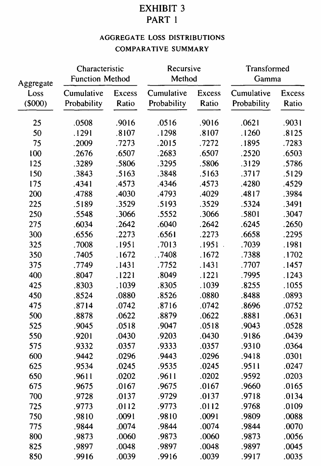
Table 5 is the whole argument of this chapter. At Venter’s $500 discretization, aggregate agrees with his recursive column to $5\times10^{-5}$ over all 34 rows, which is exact at the four decimal places printed, and differs from his characteristic function column by up to $8.2\times10^{-4}$. Refine the bucket and the two allegiances swap: by bs = 5 the agreement with the characteristic function column is $7\times10^{-5}$ and the disagreement with the recursive column has grown to $8.4\times10^{-4}$.

Venter presents two methods but we can reproduce both using FFTs at two resolutions. aggregate’s FFT with a $500 bucket agrees with the Adelson and Panjer recursion, and FFT with a $5 bucket agrees with the characteristic function inversion. The 0.0008 that Venter reports as the gap between his two exact methods is not a difference between characteristic functions and recursion at all. It is the discretization error of a $500 bucket, and it is the same error aggregate incurs when asked for the same bucket.

4.2 The excess ratio and the transformed gamma

GT(pd.DataFrame([
    {'comparison': 'agg excess ratio at bs=500 vs Venter',
     'max abs diff': float(np.abs(out['agg excess ratio']
                                  - out['Venter excess ratio']).max())},
    {'comparison': 'scipy gengamma vs Venter transformed gamma column',
     'max abs diff': float(np.abs(out['gengamma cdf']
                                  - out['Venter transf gamma']).max())},
]).set_index('comparison'), float_format=6)

Table 6: The excess ratio and transformed gamma columns, each against its published counterpart.

comparison	max abs diff
agg excess ratio at bs=500 vs Venter	0.000052
scipy gengamma vs Venter transformed gamma column	0.000049

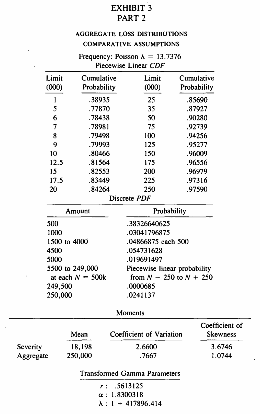
Table 6 puts both at $5\times10^{-5}$, so both columns reproduce exactly at the printed precision. The excess ratio comes straight off density_df['lev'], since $R(a) = 1 - \mathsf E[L \wedge a] / \mathsf E[L]$.

The transformed gamma check is worth doing for its own sake. Venter’s Appendix A solves two nonlinear equations in $\Gamma$ functions by Newton iteration in APL, then Exhibit 1 evaluates the incomplete gamma by a 30 to 200 term series expansion. scipy.stats.gengamma(0.5613125, 1.8300318, scale=417896.414) returns the same 34 values. The identification is exact rather than approximate: the transformed gamma with parameters $(r, \alpha, \lambda)$ is gengamma with shape $a = r$, shape $c = \alpha$ and scale $1/\lambda$.

4.3 On the approximation Venter was testing

Venter’s own verdict, that the transformed gamma is “reasonably close over a wide range of loss sizes”, reads generously with the exact answer beside it.

err = 100 * (np.array(TG) - np.array(CHAR))
inside = [x for i, x in enumerate(XS) if np.all(np.abs(err[i:]) < 0.1)]
GT(pd.DataFrame([
    {'statistic': 'largest overstatement, points of probability',
     'value': err.max(), 'at': XS[err.argmax()]},
    {'statistic': 'largest understatement, points of probability',
     'value': err.min(), 'at': XS[err.argmin()]},
    {'statistic': 'first loss size beyond which the error stays under 0.1 points',
     'value': np.nan, 'at': inside[0]},
]).set_index('statistic'), formatters={'value': 2, 'at': '{x:,.0f}'})

Table 7: How far the three-moment transformed gamma strays from the exact distribution, in points of probability.

statistic	value	at
largest overstatement, points of probability	2.53	250,000
largest understatement, points of probability	-1.60	125,000
first loss size beyond which the error stays under 0.1 points	—	725,000

By Table 7 the three-moment fit crosses the exact distribution four times over the range, running 1.1 points of probability high at $25,000, 1.6 points low at $125,000, and 2.5 points high at $250,000, its worst single row. It does not settle inside a tenth of a point until $725,000. The excess ratio column holds up better where it matters commercially, within 2% of the ratio through $650,000, before degrading to 10% at $850,000 where the ratio itself is down to 0.0039.

That is a fair result for a three-parameter fit and a poor substitute for the exact calculation, which is precisely the trade Venter names in his summary: the exact methods “require more input information … and they also require substantially more computation”, and he predicts they will become “increasingly viable” as computing gets cheaper. The four builds in this document take a few seconds each.

4.4 What did not transcribe

Figure 1 also prints Venter’s $500 discrete PDF, and I could not decode its first five rows. The rule stated for the body of that column, that the probability at $N$ is the piecewise linear probability from $N - 250$ to $N + 250$, reproduces the tabulated 0.04866875 for the $1,500 to $4,000 block exactly, but does not give the printed values at $500, $1,000, $4,500 or $5,000, and the printed $500 entry is more than twice what any nearest-bucket rule allows. Nothing here depends on it: aggregate does its own discretization from the piecewise linear CDF, and the CDF is verified independently by the three severity moments.

Venter, G. G. (1983). Transformed beta and gamma distributions and aggregate losses. Proceedings of the Casualty Actuarial Society, 70(133), 289–308.