Five papers, five programs

Author

Stephen J. Mildenhall

Published

2026-10-22 19:57 commit b5ca906+

1 How to read this chapter

This section presents a DecL solution to problems from five published results. Each has the same four parts: what the paper was doing, the exhibit it printed, the DecL program that reproduces it, and the answer beside the paper’s own numbers.

The program on each page is not typed into the page. It is read back off the object that produced the numbers, so the two cannot drift apart. Nothing else is shown, because nothing else is needed: no discretization, no grid loop, no convolution. The bucket size and the grid, the two numerical inputs that matter, are the library’s self-computed defaults in four of the five reproductions. Choosing them well is itself one of the library’s jobs, and these pages show it doing it. Venter alone states them, through the hints{} clause visible in its program, and for two reasons: his exhibit tabulates at multiples of $25,000, which the default bucket of 80 does not divide, and the argument of that section turns on comparing two deliberately chosen resolutions.

The five results are chosen to make five different points. Venter (1983) is about accuracy against a paper that computed the same thing two other ways. Bear and Nemlick (1990) shows how the library can model standard reinsurance variable features: it models six treaty features in six clauses. Homer and Clark (2003) is about reach, a joint distribution that is a view of a program rather than a second model. Bruno et al. (2006) is about speed. Denuit, Dhaene, et al. (2025) is about the reproduction checking the paper rather than the other way round, and it is the one target here that is not an insurance pricing problem at all.

The rest of this book is the detail: the transcription decisions, the readings that had to be inferred, and the cases that did not work. The detail includes a lot of Python scaffold coding that distracts from the simple DecL solution. This chapter gives just the DecL highlights and omits the scaffolding.

Exception reporting mode: Minimal

2 Venter (PCAS, 1983): Transformed Beta And Gamma Distributions And Aggregate Losses

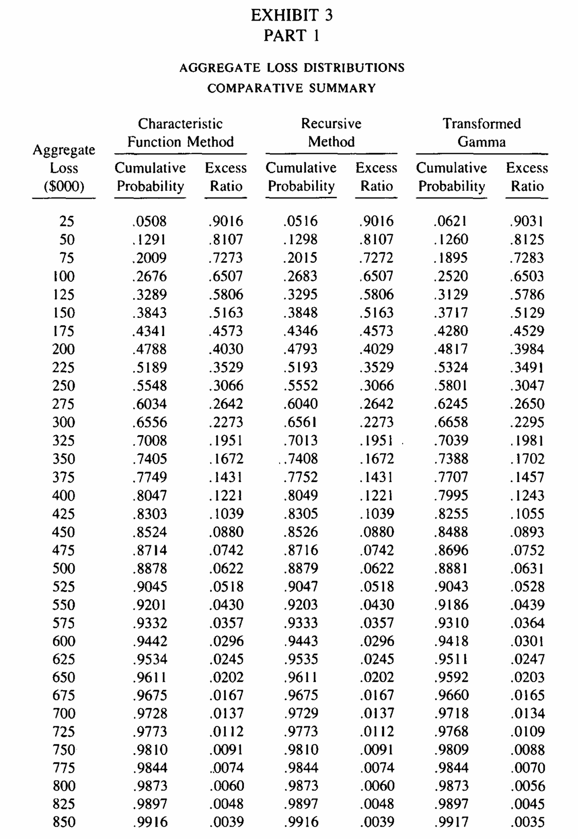
Venter (1983) introduced the transformed gamma to actuarial work and closed by testing it against the exact aggregate distribution. His Exhibit 3 computes the cumulative probability distribution of one compound Poisson three ways over $25,000 to $850,000: by characteristic function inversion, by the Adelson and Panjer recursion, and by a transformed gamma matched to three moments, see Figure 1. Frequency is Poisson with $\lambda = 13.7376$ and severity is a piecewise linear claim size CDF to a $250,000 policy limit, tabulated at 23 points.

Figure 1: Venter (1983), Exhibit 3, Part 1.

V:\worktrees\aggregate_REFACTOR\src\aggregate\_aggregate.py:4481: DefectiveDistributionWarning: Venter: aggregate PMF deficit 1.302e-04 (Σp = 1 − 1.302e-04 < 1); forwards and backwards S diverge by the deficit (forwards > backwards). Further occurrences this session are suppressed; each object records its own verdict in validation.
  rv = self.update_work(xs, debug=debug, x_min=x_min, x_max=x_max,

agg Venter
  13.7376 claims
  250000 xs 0
  sev chistogram xps [0 1000 5000 6000 7000 8000 9000 10000 12500 15000 17500 20000 25000 35000 50000 75000 100000 125000 150000 175000 200000 225000 250000 300000] [0.38935 0.38935 0.00568 0.00543 0.00517 0.00495 0.00473 0.01098 0.00989 0.00896 0.00815 0.01426 0.02237 0.02353 0.02459 0.01517 0.01021 0.00732 0.00547 0.00423 0.00337 0.00274 0.0241]
  poisson
  hints{log2=16; bs=500; normalize=False; padding=1}

The small bucket size does not have full extent and triggers the (harmless) DefectiveDistributionWarning. The validation explains.

print(textwrap.fill(v5.validation_explanation, 72))

Validation of the realized grid against the analytic moments: fails pmf
deficit 1.302e-04. Each of mean, CV and skewness is compared for
severity and for the aggregate, and a relative error above 0.0001 fails;
only the lowest-order failure is reported, since a mean that is wrong
makes the higher moments uninformative. The realized law does not sum to
1: 1.302e-04 of the probability ran off the top of the grid and was
dropped rather than wrapped. Forwards S = 1 - cumsum carries the missing
mass as a tail blob and backwards S drops it, so the two pricing routes
disagree by exactly this amount and neither is wrong. Raise log2, or
widen the grid.

Table 1: Validation of part of Venter Exhibit 3, Part 1.

aggregate loss	Venter char fn	Venter recursive	agg bs=500	agg bs=5	agg bs=100.0
225,000	0.5189	0.5193	0.5193	0.5189	0.5190
250,000	0.5548	0.5552	0.5552	0.5548	0.5549
275,000	0.6034	0.6040	0.6040	0.6034	0.6035
300,000	0.6556	0.6561	0.6561	0.6556	0.6557
325,000	0.7008	0.7013	0.7013	0.7008	0.7009
350,000	0.7405	0.7408	0.7408	0.7405	0.7405
375,000	0.7749	0.7752	0.7752	0.7749	0.7750
400,000	0.8047	0.8049	0.8049	0.8047	0.8047

Table 1 shows eight of the thirty four rows, at the middle of the range. Table 2 measures the fit over all thirty four.

Table 2: Largest absolute difference from each of Venter’s two exact columns, over the full range.

rows compared	agg bs=500 vs his recursive column	agg bs=5 vs his characteristic function column
34	5.1e-05	7.3e-05

Venter presents two exact methods that differ by up to 0.0008, and reads that gap as the cost of discretizing severity. Forty years later we can reproduce both with one method using two resolutions. Change bs=500 to bs=5, one token in one program, and aggregate stops agreeing with his recursion and starts agreeing with his characteristic function instead. The 0.0008 was never a difference between the methods. It was the $500 bucket, and it is the same error aggregate incurs when asked for the same bucket.

3 Bear and Nemlick (1990): six treaty features, six clauses

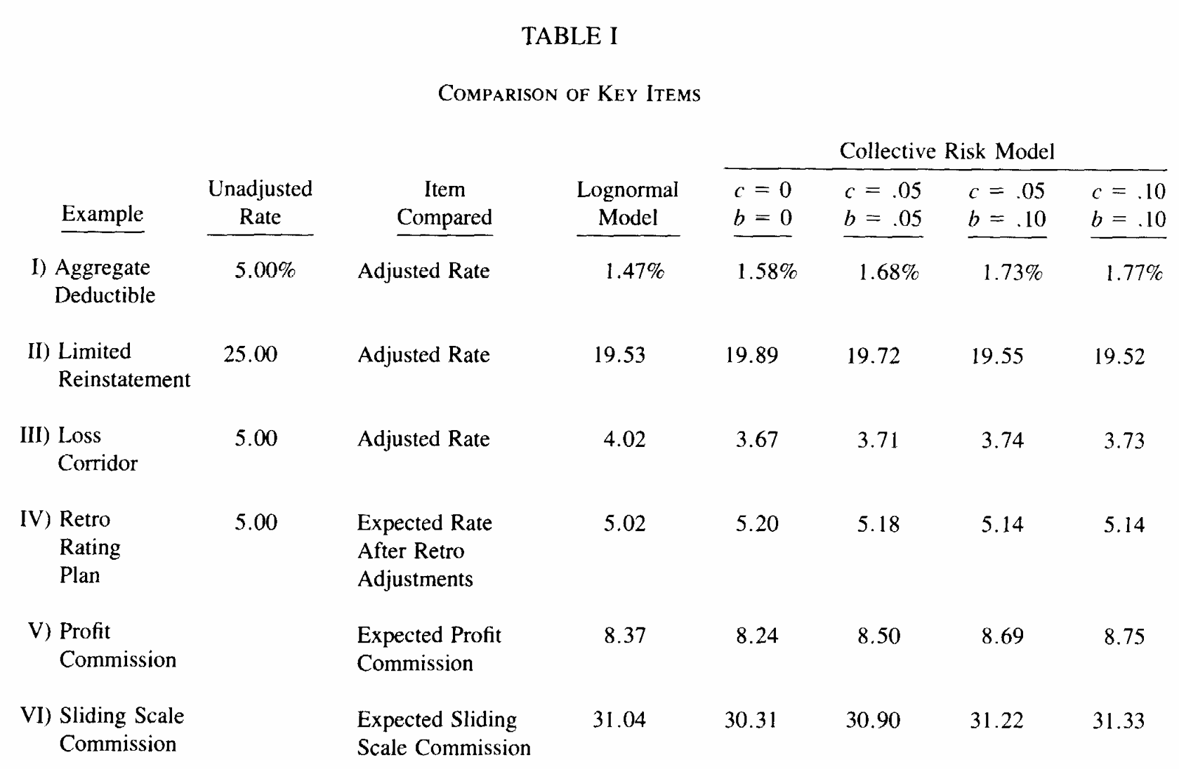
Bear and Nemlick (1990) price six reinsurance treaties that each carry one adjustable feature, comparing a lognormal approximation of the aggregate against the collective risk model. Their Table I, Figure 2, shows the six answers. The subject book is two excess casualty classes written at $160,000 xs 0 with Pareto severities and gamma mixed Poisson counts. Treaty I puts an annual aggregate deductible of $360,000 against $450,000 of expected layer loss, an entry ratio of 0.800, and the indicated rate is the loss cost surviving the deductible loaded 100/75.

Figure 2: Bear and Nemlick (1990), Table I.

agg BN.One
  [9000 3000] premium at [0.04 0.03] lr
  160 xs 0
  sev 40 * pareto [0.9 0.95] + -40
  poisson
  aggregate net of
    360 xs 0

An aggregate deductible is an aggregate layer the cedant keeps, so the recovery is the aggregate net of it, and the whole feature is the last clause. Nothing else in the program changes.

Table 3: Treaty I, the annual aggregate deductible, against the two columns of Table I.

expected layer loss, 000s	insurance charge, exact	indicated rate %, agg	Table I, collective risk	Table I, lognormal
450.0	0.3151	1.5755	1.580	1.470

In Table 3 the exact answer is 1.5755% against 1.58% printed, and the lognormal shortcut the paper was testing reads 1.47%. The other five treaties are one clause each, as Table 4 sets out, and the detail chapter prices all six.

Table 4: The adjustable feature of each Bear and Nemlick treaty, and the DecL clause that expresses it.

Treaty	Feature	DecL clause
I	annual aggregate deductible	`aggregate net of 360 xs 0`
II	three free reinstatements	`reinstatements 3 free`
III	loss corridor	`corridor`
IV	retrospective rating	`retro`
V	three year profit commission	`pc`
VI	sliding scale commission	`slide`

Six treaties, six clauses, and no arithmetic outside the loading factors the slips specify. The detail chapter reproduces the lognormal column exactly at every printed digit and the collective risk column to the printed digit in five of the six.

Here are all six programs, at Poisson counts, as the detail chapter writes them. They are worth reading side by side: every one is the same shape, a subject book with a feature clause on the end, and the differences between the six treaties are differences of one clause. Five wrap in an xpnl, the walk face, which books each cession as its own step so the recovery, the ceded premium and any commission come back as separate legs. Treaty IV uses pnl instead, because a retro plan varies the gross premium rather than ceding anything, so there is no cession to walk and the plan replaces the premium at the head of the program.

These are shown as authored rather than as parsed, which is the one place in this chapter where that distinction matters. The canonical form the parser renders back spells several of these clauses differently: reinstatements 3 free is stored as a vector of three zero charges and comes back reinstatements [0 0 0], percentages resolve to decimals so corridor 100% po 100% xs 100% comes back corridor 1 po 1 xs 1, and exposure at rate and premium at lr are one construct with premium as the canonical spelling. Everything downstream is driven by the parse, not by this text. The slip language is what is worth reading here.

Treaty I: annual aggregate deductible

agg BN.One [9000 3000] exposure at [0.04 0.03] rate 160 xs 0
    sev 40 * pareto [0.90 0.95] - 40
    poisson
    aggregate net of 360 xs 0

Treaty II: three free reinstatements

xpnl BN.TreatyII 1172 premium less
    agg BN.Two [2000 2000 2000] exposure at [0.10 0.14 0.21] rate 700 xs 0
        sev 300 * pareto [1.5 1.3 1.1] - 300
        occurrence net of 700 xs 0 deposit 1172 reinstatements 3 free as "Layer"
        poisson

Treaty III: loss corridor

xpnl BN.TreatyIII 10000 premium less
    agg BN.Three [4500 4500 1000] exposure at [0.032 0.038 0.035] rate 400 xs 0
        sev 100 * pareto 1.1 - 100
        poisson
        aggregate net of 10000 xs 0 deposit 350
                       corridor 100% po 100% xs 100% as "Corridor"

Treaty IV: retrospective rating

pnl BN.TreatyIV retro basic 0 lcm 1.3333333333 min 360 max 1200 premium less
    agg BN.Four [9000 3000] exposure at [0.04 0.03] rate 160 xs 0
        sev 40 * pareto [0.90 0.95] - 40
        poisson

Treaty V: three year profit commission

xpnl BN.TreatyV 18000 premium less
    agg BN.Five [6000 6000 6000] exposure at [0.10 0.14 0.21] rate 700 xs 0
        sev 300 * pareto [1.5 1.3 1.1] - 300
        poisson
        aggregate net of 80% po 100000 xs 0 deposit 5625
                       pc 25% after 20% as "PC layer"

Treaty VI: sliding scale commission

xpnl BN.TreatyVI 25000 premium less
    agg BN.Six 25000 exposure at 0.10 rate 900 xs 0
        sev 100 * pareto 0.98 - 100
        poisson
        aggregate net of 100000 xs 0 deposit 5000
                       slide 40% at 35% and 25% at 55% and 20% at 65% as "Slide"

Three details these programs make visible that the prose above glosses over. The nominal wide layers in III, V and VI (10000 xs 0, 100000 xs 0) are not terms of the treaty: a decorator clause has to sit on an aggregate layer, so the layer is written high enough to reach everything the aggregate does and the feature supplies the only binding term. The deposit in each is the base premium the feature prices against, which is why the corridor’s 100% po 100% xs 100% reads in loss ratio points exactly as the slip does. And the 80% po in Treaty V is a placement rather than a cession: premium clauses are quoted at 100% and scaled by the fraction placed, so the slip’s $4,500 on an 80% placement is a deposit of $5,625.

The one genuine constraint is that each program carries exactly one feature. Three of the five features read a ceded loss ratio, and that ratio is only a deterministic rescaling of the ceded loss while the denominator stays fixed. Put two features on one program and the second reads a random denominator. The paper reaches the same conclusion from the other side in its section 5, and proposes running the collective risk model a second time on the post-coinsurance distribution: a two stage construction, not a single decorated layer.

4 Homer and Clark (2003): the joint distribution is a view, not a second model

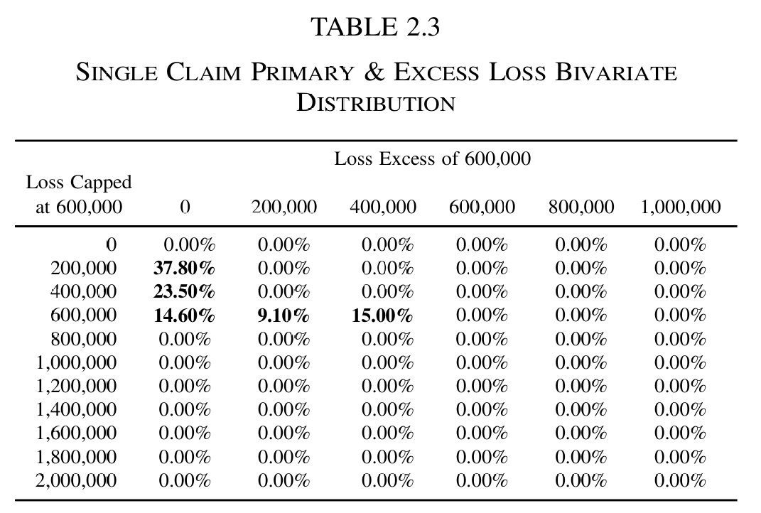
Homer and Clark (2003) introduces the two dimensional FFT to actuarial work, for the case where two covers on the same book are driven by the same losses and so cannot be priced separately. Section 2 retains $600,000 per occurrence, buys $400,000 xs $600,000 per occurrence, and puts a $5,000,000 xs $3,000,000 stop loss on the retention. The paper builds the joint law of retained and ceded by hand, as its Table 2.3, Figure 3.

Figure 3: Homer and Clark (2003), Table 2.3.

agg HC
  5 claims
  dsev [200000 400000 600000 800000 1000000] [0.378 0.235 0.146 0.091 0.15]
  occurrence net of
    400000 xs 600000
  mixed gamma 0.2

That program declares the treaty and nothing two dimensional. Retained and ceded are the net and ceded views of an occurrence layer already in it, so the joint severity is the cession map applied to the gross severity, and the joint distribution is one call away: a.occ_bivariate(views=('net', 'ceded')). The paper’s Table 2.3 falls out as a by-product rather than an input.

Table 5: The five statistics Homer and Clark read off Table 2.3, taken instead from the bivariate view of the program.

statistic	aggregate	paper
expected loss to the stop loss layer	123,529.2617	123,529.0000
probability the stop loss is hit	0.1508	0.1508
mean stop loss given it is hit	819,209.9114	819,210.0000
expected loss to the per-occurrence layer	390,999.9993	391,000.0000
expected per-occurrence loss given the stop loss is hit	830,334.0200	830,334.0000

Table 5 reproduces all five to the digit, and the last two are the paper’s point. The per-occurrence layer costs $391,000 on average but $830,334 in the scenarios where the stop loss also pays. Writing both covers is more than twice as bad as the two expected values suggest, and that is invisible to anyone pricing them separately.

5 Bruno, Camerini, Manna and Tomassetti (2006): 92,832 convolutions

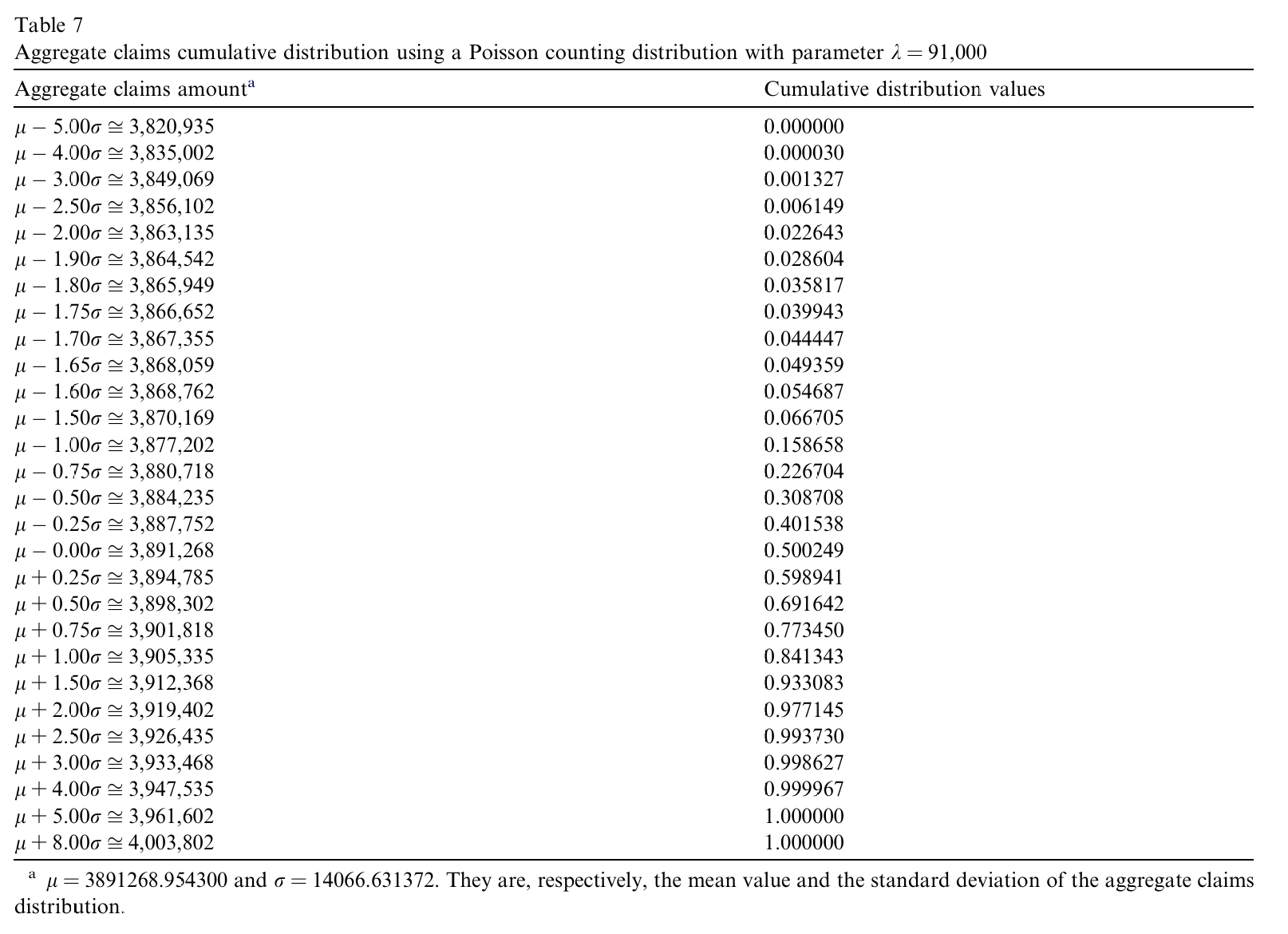
Bruno et al. (2006) proposes thresholded direct convolution as a cheaper alternative to Panjer recursion, De Pril transforms and the FFT. Table 7, Figure 4, is the showcase: a Poisson with $\lambda = 91{,}000$ against a fourteen point discrete severity, which their formalization reaches in 92,832 convolutions. Table 4 records that Panjer recursion and De Pril both underflow at $\lambda$ as low as 1,004.8, that their own method took 1,950 seconds here, and that their FFT comparison stopped at $\lambda = 5{,}004.8$ after 3,850 seconds.

agg B7
  91000 claims
  dsev [14 15 16 17 18 19 20 24 26 28 30 31 55 60] [0.0103301 0.030799 0.0293511 0.0103301 0.0730414 0.0111568 0.0264554 0.1002133 0.0815418 0.0252146 0.0212857 0.0254214 0.0991756 0.4556837]
  poisson

The program carries no hints{} clause, so the grid is the library’s own. That is possible because the aggregate is computed in its support window rather than from zero, and at $\lambda = 91{,}000$ that window is a narrow interval around a mean of 3.89 million. Table 7 reports the grid the library chose for it, and the whole of Table 7 comes back exact on that grid.

Table 6: Eight of the twenty eight aggregate loss points Table 7 prints, against the program’s CDF.

aggregate loss	agg CDF	Table 7 CDF
3,877,202	0.158658	0.158658
3,880,718	0.226704	0.226704
3,884,235	0.308708	0.308708
3,887,752	0.401538	0.401538
3,891,268	0.500249	0.500249
3,894,785	0.598941	0.598941
3,898,302	0.691642	0.691642
3,901,818	0.773450	0.773450

Table 6 shows eight of the printed points; Table 7 takes in all of them, and the clock.

Table 7: Accuracy over all twenty eight rows, and the run time beside the paper’s own.

rows compared	largest CDF difference	aggregate seconds	paper seconds	grid points	mean	paper mean
28	4.8e-07	0.10000	1,950	262,144	3,891,268.9543	3,891,268.9543

All twenty eight published values are exact at the six decimals printed. The paper counted the FFT as one transform per convolution and summed over 92,832 of them, which is not how a compound distribution is computed: the frequency enters through its probability generating function applied pointwise to the severity transform, so the whole distribution costs two transforms whether $\lambda$ is 500 or 91,000. Some of the timing gap is twenty years of hardware but that structural part is not.

6 Denuit, Dhaene, Ghossoub and Robert (2025): the check runs both ways

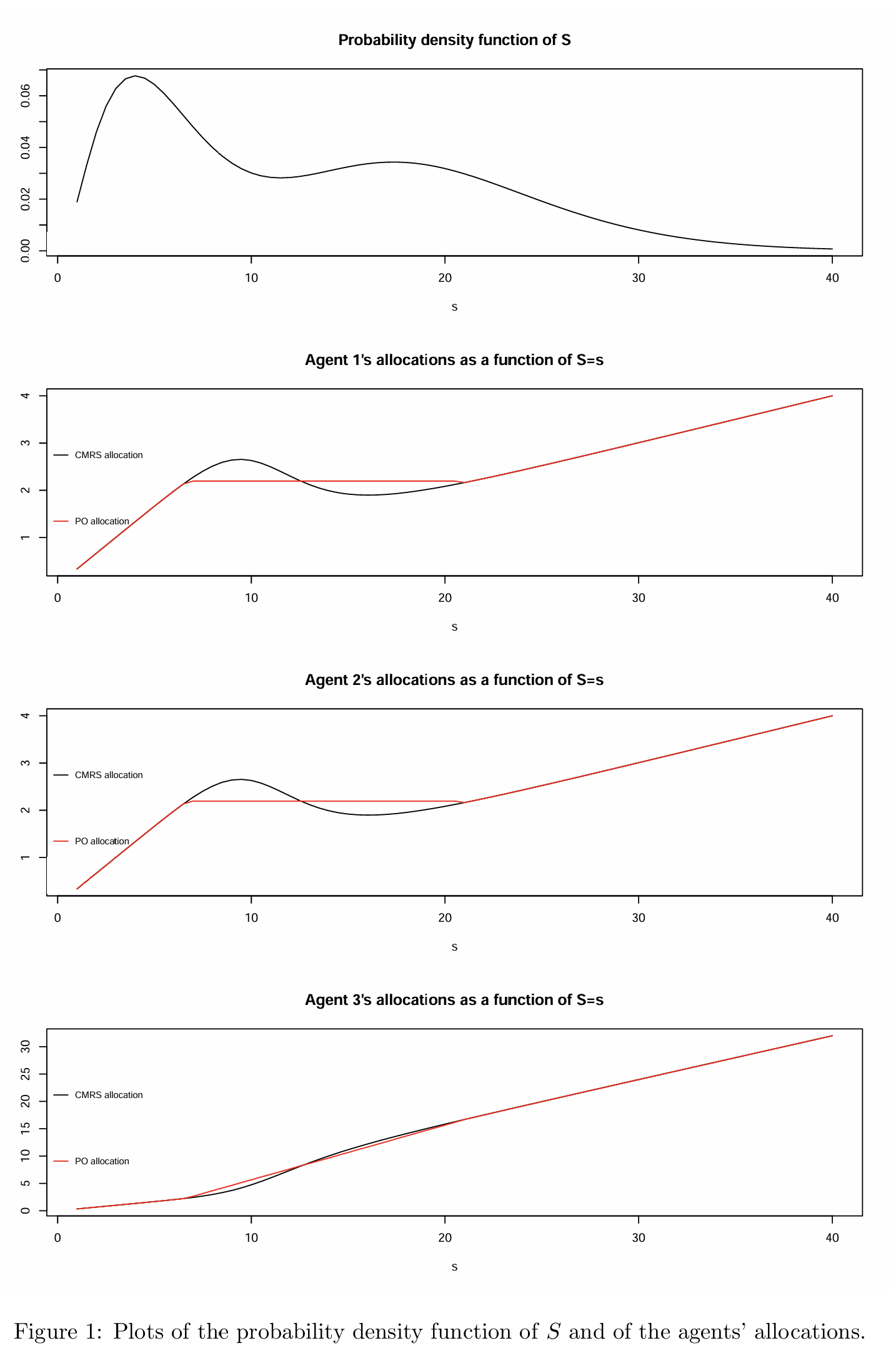
Denuit, Dhaene, et al. (2025) settle a question about risk sharing rather than insurance pricing. Given a pool of losses $S = X_1 + \dots + X_n$, the conditional mean risk sharing rule allocates $\kappa_i(s) = \mathsf E[X_i \mid S = s]$ to agent $i$. That rule is not always comonotonic: an agent’s share can fall as the pool’s total loss rises, which violates the no-sabotage condition and is not Pareto optimal for the convex order. The paper’s contribution is an explicit algorithm, from majorization theory, that converts any such allocation into a comonotonic one that improves every agent in convex order while preserving every expectation. Its section 3.2 example is three independent agents: agents 1 and 2 carry a truncated exponential on $[0, 10]$ with $\beta = 1/2$, and agent 3 a truncated equal mixture of an exponential and a $\Gamma(8)$ on $[0, 30]$.

This is a natural reproduction target because $\kappa_i$ is not a special quantity here. It is the exeqa_ column of a portfolio’s density_df, the same conditional expectation aggregate uses for capital allocation, and the paper’s algorithm ships as Portfolio.make_comonotonic_allocations. Figure 5 is the target.

Figure 5: Denuit, Dhaene, Ghossoub and Robert (2025), Figure 1.

port Denuit.Pool
  agg Agent1
    1 claim
    sev 2 * expon splice [0 10]
    fixed
  agg Agent2
    1 claim
    sev 2 * expon splice [0 10]
    fixed
  agg Agent3
    1 claim
    sev 2 * gamma [1 8] wts [0.504541349633 0.495458650367] splice [0 0] [30 30]
    fixed

A truncated distribution is a splice, and the mixture is a two component severity, so the whole three agent pool is one portfolio declaration. Before reading any allocation, check the model against the paper’s own specification, which Table 8 does.

Table 8: The pool’s means against direct quadrature on the paper’s own specification.

quantity	quadrature	aggregate
E[X_1], truncated exponential on [0, 10]	1.93216345	1.93216337
E[X_3], truncated mixture on [0, 30]	8.77944917	8.77944913
E[S]	12.64377607	12.64377587

Two structural facts follow from the specification and hold to numerical precision in Table 9, which is what says the pool is built right. Agents 1 and 2 are identically distributed, so $\kappa_1 \equiv \kappa_2$; and an allocation adds up, so $\sum_i \kappa_i(s) = s$ at every $s$.

Table 9: The two structural invariants, symmetry of agents 1 and 2 and adding up, at numerical precision.

$\max \|\kappa_1 - \kappa_2\|$ over $s \in [0.5, 45]$	$\max \|\sum \kappa_i - s\|$
0.0e+00	1.1e-10

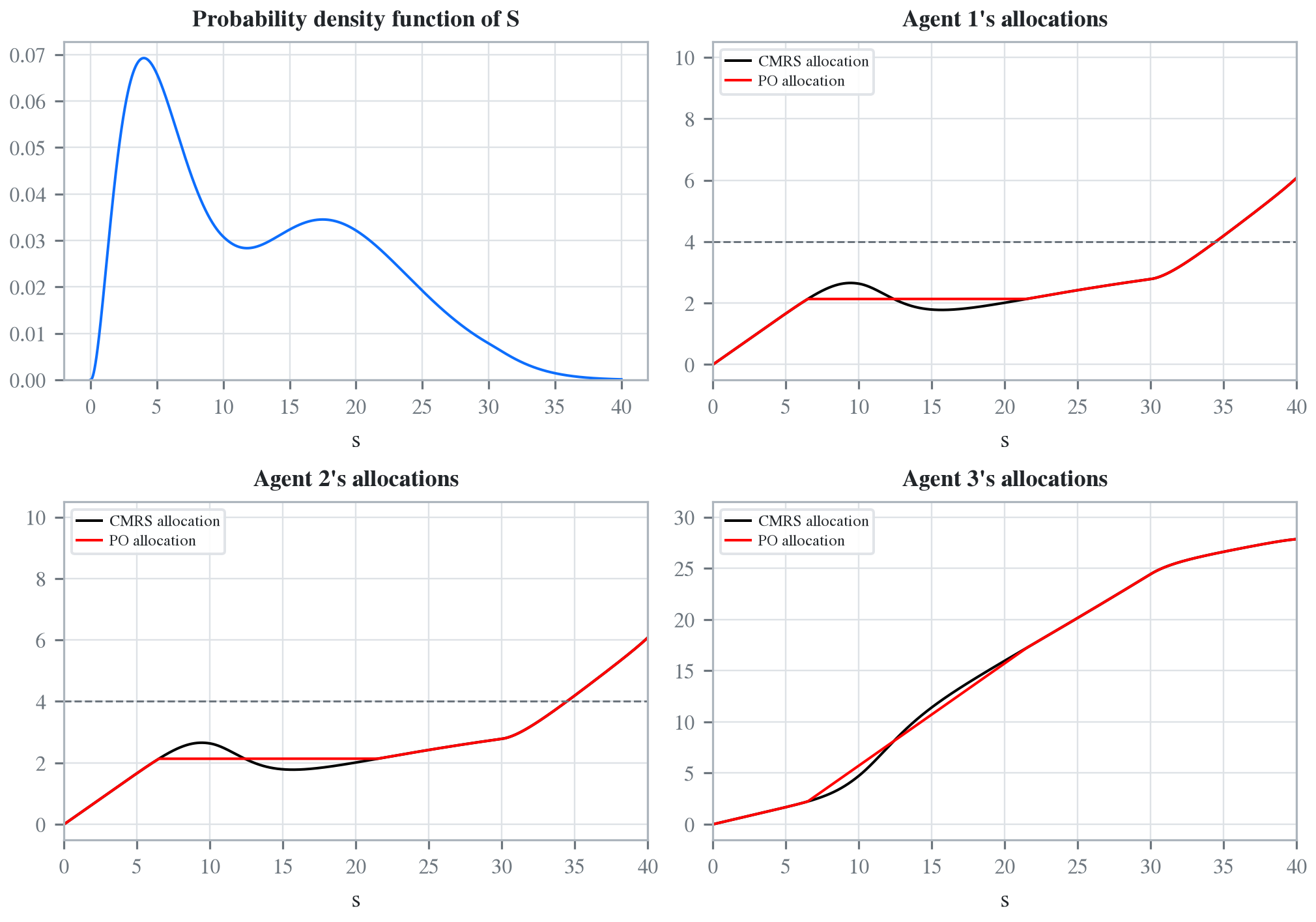
Now the figure, Figure 6. The black curves are the conditional mean allocations, the red the comonotonic Pareto optimal improvement from the paper’s algorithm.

Figure 6: Reproducing Figure 1. The dashed line on the agent 1 and 2 panels is the top of the published axis.

Table 10: The conditional mean allocations at seven values of the pool total, showing the non-monotone stretch.

s	$\kappa_1 = \kappa_2$	$\kappa_3$	sum
10	2.63104	4.73793	10.00000
15	1.78877	11.42245	15.00000
20	2.01153	15.97694	20.00000
25	2.42093	20.15814	25.00000
30	2.78147	24.43705	30.00000
35	4.19309	26.61381	35.00000
40	6.07707	27.84586	40.00000

The paper’s qualitative claim reproduces exactly in Table 10: $\kappa_1$ and $\kappa_2$ rise to 2.63 at $s = 10$, fall to 1.79 by $s = 15$, and rise thereafter, so the conditional mean allocation is not comonotonic and not Pareto optimal, and the algorithm flattens precisely that stretch.

The published Figure 5 cannot be right at its own right hand edge, and it takes no computation to see why. Agent 3’s loss is capped at $N = 30$, so at $s = 40$ adding up forces $\kappa_1 + \kappa_2 \ge 10$, and by symmetry $\kappa_1 = \kappa_2 \ge 5$. The published panels for agents 1 and 2 are drawn on an axis whose top tick is 4. The true values are $\kappa_1(35) = 4.19$ and $\kappa_1(40) = 6.08$, which leave the box. Dropping the $N = 30$ truncation of agent 3, and only that, brings $\kappa_1(40)$ down to 3.31 and inside it, which is the one reading of the model consistent with what is printed.

Nothing in the paper’s theorems depends on this. The algorithm is right, the code that ships it here is the paper’s, and the interesting part of Figure 5, the non-monotone stretch the algorithm exists to repair, is exactly where the paper says it is.

7 Where the detail is

Each of these has a chapter, and the chapters carry what a page cannot: the transcription decisions, the readings that had to be inferred and then confirmed by fit, the grid caveats, and the arithmetic behind every acceptance test. Venter (1983), Bear and Nemlick (1990) and Homer and Clark (2003) are in the actuarial models part, Bruno et al. (2006) in the part on exact computation, and Denuit, Dhaene, et al. (2025) sits with Denuit, Ortega-Jiménez, et al. (2025) in the part on conditional expectations given the sum.

The book also carries what did not work, which is the more informative half. Jin et al. (2016) has a part to itself and is not a reproduction: the feature it needs, common shock dependence on frequencies rather than on a joint severity, does not exist. Ben Rached et al. (2024) and Wilson and Keich (2016) locate a floor under FFT accuracy, below roughly $10^{-13}$, and Wilson and Keich (2017) shows the repair. Three of the fifteen papers contain errors the reproduction found, which is not a criticism of the authors so much as evidence that the check runs in both directions.

Programs in the aggregate Loss Lab

Each program below opens in the aggregate Loss Lab, which builds it with nothing to install. The names are those in reproductions.agg, where every program is renamed by its paper’s citation key.

Venter1983.Venter: Exhibit 3, a compound Poisson over a tabulated claim size law.
Bear1990.BN.One: the subject book of two excess casualty classes.
Bear1990.BN.One.v2: Treaty I, an annual aggregate deductible on the subject book.
Homer2003.HC: Section 2's per occurrence layer, whose net and ceded views give Table 2.3.
Bruno2006.B7: Table 7's compound Poisson at lambda = 91,000.
Denuit2025a.Denuit.Pool: Section 3.2's three agent pool of truncated severities.

Bear, R. A., & Nemlick, K. J. (1990). Pricing the impact of adjustable features and loss sharing provisions of reinsurance treaties. Proceedings of the Casualty Actuarial Society, 77(147), 86–87. https://doi.org/10.1016/0167-6687(93)91078-9

Ben Rached, N., Hoel, H., & Meo, J. V. (2024). A fast and accurate numerical method for the left tail of sums of independent random variables. Statistics and Computing. https://doi.org/10.1007/s11222-024-10514-5

Bruno, M. G., Camerini, E., Manna, A., & Tomassetti, A. (2006). A new method for evaluating the distribution of aggregate claims. Applied Mathematics and Computation. https://doi.org/10.1016/j.amc.2005.09.038

Denuit, M. M., Dhaene, J., Ghossoub, M., & Robert, C. Y. (2025). Comonotonicity and Pareto optimality, with application to collaborative insurance. Insurance: Mathematics and Economics, 120, 1–16. https://doi.org/10.1016/j.insmatheco.2024.11.001

Denuit, M. M., Ortega-Jiménez, P., & Robert, C.-Y. (2025). Conditional expectations given the sum of independent random variables with regularly varying densities. ASTIN Bulletin. https://doi.org/10.1017/asb.2025.11

Homer, D. L., & Clark, D. R. (2003). Insurance Applications of Bivariate Distributions. Proceedings of the Casualty Actuarial Society, 90(iid), 274–307. http://www.casact.org/pubs/proceed/proceed03/03274.pdf

Jin, T., Provost, S. B., & Ren, J. (2016). Moment-based density approximations for aggregate losses. Scandinavian Actuarial Journal, 2016(3), 216–245. https://doi.org/10.1080/03461238.2014.921640

Venter, G. G. (1983). Transformed beta and gamma distributions and aggregate losses. Proceedings of the Casualty Actuarial Society, 70(133), 289–308.

Wilson, H., & Keich, U. (2016). Accurate pairwise convolutions of non-negative vectors via FFT. Computational Statistics and Data Analysis, 101, 300–315. https://doi.org/10.1016/j.csda.2016.03.010

Wilson, H., & Keich, U. (2017). Accurate small tail probabilities of sums of iid lattice-valued random variables via FFT. Journal of Computational and Graphical Statistics, 26(1), 223–229.