Embrechts, Grübel and Pitts on discretization error
Reproducing Embrechts, Grübel and Pitts (1993)
Author
Stephen J. Mildenhall
Published
2026-10-22 19:55 commit b5ca906+
1 Context and problem
Every FFT aggregate begins by replacing a continuous severity with a lattice distribution of span \(h\). That step costs accuracy, and the cost is separate from aliasing: it would be there on an infinitely long grid with no wraparound at all. Embrechts et al. (1993) is the paper that identified the rate at which it goes away, and then removed most of it for free.
The mechanism is Richardson’s deferred approach to the limit, standard in numerical analysis and unfamiliar in actuarial work. Suppose an estimator satisfies
The leading error term is gone and the constant \(c_1\) never had to be known. All that is needed is \(\alpha\).
The paper’s contribution is to establish \(\alpha = 2\) for compound distributions. Its Theorem shows that under smoothness conditions on the severity density and the integrand,
for an explicit \(H\), so the discretization error is exactly \(O(h^2)\) and \(t = 2\) gives the familiar combination \((4 I(h/2) - I(h))/3\).
2 Paper solution and gold standard
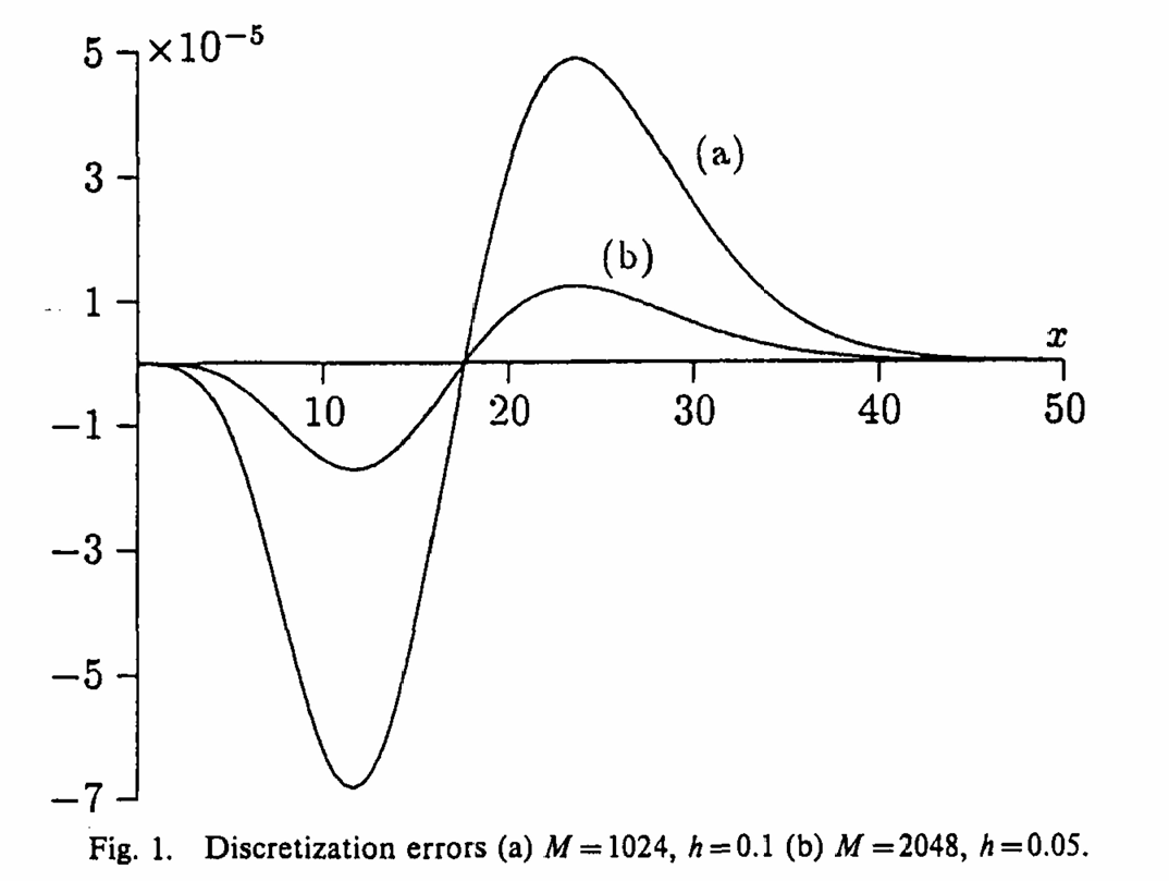
Figure 1, Figure 1, is the illustration, and its caption gives the whole specification: claim sizes exponential with mean 1, claim count Poisson with mean 20, and two discretizations, (a) \(M = 1024\), \(h = 0.1\) and (b) \(M = 2048\), \(h = 0.05\). Both reach the same truncation point, \(Mh = 102.4\), which is the point: they differ only in span.
Section 5 then combines the two density estimates \(g_{M,k}/h\) and \(g_{2M,2k}/h\) into
and reports that “the error associated with this approximation is also displayed, it is indistinguishable from the horizontal axis”. The paper adds the honest caveat that this particular application, a density rather than an integral \(\int \phi\,\mathrm dG\), is not covered by its own Theorem.
So there are two things to check and no table to check them against: that the error really is \(O(h^2)\), and that the extrapolation really is invisible on the same axis.
2.1 The gold standard here is exact
This example has a closed-form answer, which is unusual and makes the reproduction much sharper than a comparison against a finer grid. A compound Poisson with exponential severity has density
with \(I_1\) the modified Bessel function of the first kind, plus an atom of \(e^{-\lambda}\) at zero. So the discretization error can be measured rather than estimated, once Table 1 confirms the closed form is the right function.
%xmode minimalimport numpy as npimport pandas as pdimport matplotlib.pyplot as pltfrom scipy.special import i1efrom aggregate.constants import FIG_W, FIG_Hfrom bookstyle import GT, build, showLAM, BETA =20.0, 1.0def exact_density(x):"""Closed-form compound Poisson-exponential density. Zero at x <= 0.""" x = np.asarray(x, dtype=float) out = np.zeros_like(x) m = x >0 z =2* np.sqrt(LAM * BETA * x[m])# i1e(z) = I_1(z) e^{-z}; fold the exponent in to stay in range out[m] = (np.exp(-LAM - BETA * x[m] + z)* np.sqrt(LAM * BETA / x[m]) * i1e(z))return outxx = np.linspace(1e-9, 400, 4_000_001)fx = exact_density(xx)GT(pd.DataFrame([ {'quantity': 'integral of the closed-form density', 'value': float(np.trapezoid(fx, xx)),'exact': 1- np.exp(-LAM)}, {'quantity': 'its first moment', 'value': float(np.trapezoid(xx * fx, xx)),'exact': LAM / BETA},]).set_index('quantity'), float_format=10)
Exception reporting mode: Minimal
Table 1: The closed form density integrated and its first moment, against their exact values.
quantity
value
exact
integral of the closed-form density
0.9999999979
0.9999999979
its first moment
20.0000000000
20.0000000000
In Table 1 it integrates to \(1 - e^{-20}\), the probability of at least one claim, and has mean 20. It is the right function.
3 The aggregate reproduction
def egp(M, h):return build(f'agg EGP {LAM:g} claims sev expon {1/BETA:g} poisson 'f'hints{{log2={int(np.log2(M))}; bs={h}; padding=1; normalize=False}}')CASES = {'(a) M = 1024, h = 0.1': (1024, 0.1), '(b) M = 2048, h = 0.05': (2048, 0.05)}objs = {k: egp(M, h) for k, (M, h) in CASES.items()}show(objs['(a) M = 1024, h = 0.1'])
Table 2 records both builds and their shared truncation point.
rows = []for k, (M, h) in CASES.items(): a = objs[k] rows.append({'case': k, 'M': M, 'h': h, 'truncation point M h': M * h,'E[S] agg': a.est_m, 'E[S] exact': LAM / BETA,'total mass': a.agg_density.sum()})GT(pd.DataFrame(rows).set_index('case'), formatters={'M': 0, 'h': '{x:g}', 'truncation point M h': 1,'E[S] agg': 6, 'E[S] exact': 6, 'total mass': 10})
Table 2: The paper’s two discretizations, sharing a truncation point and differing only in span.
case
M
h
truncation point M h
E[S] agg
E[S] exact
total mass
(a) M = 1024, h = 0.1
1,024
0.1
102.4
19.991669
20.000000
1.0000000000
(b) M = 2048, h = 0.05
2,048
0.05
102.4
19.997917
20.000000
1.0000000000
3.1 Figure 1
Table 3 measures both of the paper’s claims at once.
dens = {}for k, (M, h) in CASES.items(): a = objs[k] x = a.density_df.index.to_numpy() dens[k] = (x, a.density_df.p_total.to_numpy() / h)xc, dc = dens['(a) M = 1024, h = 0.1']xf, df_ = dens['(b) M = 2048, h = 0.05']d_fine_on_coarse = df_[::2][:len(dc)] # every other fine pointrich = (4* d_fine_on_coarse - dc) /3# the paper's combinationex = exact_density(xc)sl = (xc >0) & (xc <=60)err = pd.DataFrame({'h = 0.1': dc[sl] - ex[sl],'h = 0.05': d_fine_on_coarse[sl] - ex[sl],'Richardson': rich[sl] - ex[sl]}, index=xc[sl])GT(pd.DataFrame([ {'estimate': c, 'max |error| on (0, 60]': float(err[c].abs().max())}for c in err.columns] + [ {'estimate': 'ratio, h = 0.1 over h = 0.05','max |error| on (0, 60]': float(err['h = 0.1'].abs().max()/ err['h = 0.05'].abs().max())}]).set_index('estimate'), formatters={'max |error| on (0, 60]': '{x:.4e}'})
Table 3: Worst density error at each span and for the Richardson combination, with the ratio between the two spans.
estimate
max |error| on (0, 60]
h = 0.1
6.8213e-05
h = 0.05
1.7060e-05
Richardson
1.9350e-08
ratio, h = 0.1 over h = 0.05
3.9984e+00
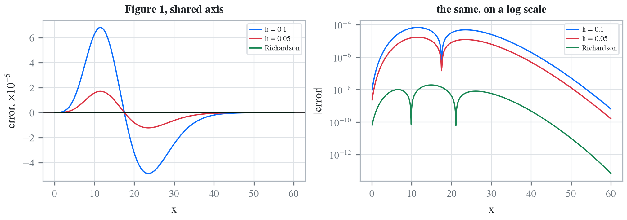
Both of the paper’s claims hold in Table 3. The error ratio between \(h = 0.1\) and \(h = 0.05\) is 3.998, which is the paper’s Theorem measured rather than assumed: halving the span quarters the error, so \(\alpha = 2\). And the extrapolated error is \(1.9\times10^{-8}\) against \(6.8\times10^{-5}\) for the coarse estimate, a factor of 3,525, so on a shared axis it is indeed indistinguishable from zero.
Figure 1: Embrechts, Grübel and Pitts (1993), Figure 1.
Figure 2: Reproducing Figure 1. Discretization error of the density estimate at h = 0.1 and h = 0.05, and of the Richardson combination of the two.
The left panel of Figure 2 is the paper’s figure: two visible error curves and a third lying on the axis. The right panel is the part a shared linear axis cannot show, which is that the Richardson curve is not merely small but three orders of magnitude below the inputs it was built from, uniformly across the range.
3.2 The same thing on a scalar
The density is not covered by the paper’s Theorem, as it says. The mean is, and Table 4 makes the point in one line, since \(\mathsf E[S] = 20\) exactly.
Table 4: The aggregate mean at each span and after extrapolation, against the exact value of 20.
estimate
E[S]
error
h = 0.1
19.991669097
-8.331e-03
h = 0.05
19.997916819
-2.083e-03
Richardson, (4 fine - coarse) / 3
19.999999393
-6.074e-07
In Table 4 the two mean errors are \(-8.33\times10^{-3}\) and \(-2.08\times10^{-3}\), in the ratio 4.000, and the extrapolation lands within \(3\times10^{-7}\) of 20. Here the \(O(h^2)\) behaviour is not empirical: the rounding discretization has a known bias, and the extrapolation cancels it to the order the Theorem predicts.
4 Comments
4.1 What Richardson buys, and when it is the wrong tool
The extrapolation above cost one extra build and bought three orders of magnitude. Simply refining to \(h = 0.05\) cost the same extra build and bought a factor of four. On this example the extrapolation wins overwhelmingly, and the reason is that the error is clean: it is dominated by a single \(h^2\) term with a smooth coefficient, which is precisely the situation the Theorem describes.
It stops working when that premise fails, and there are two ordinary ways for it to fail. If the severity has a jump or a kink, the density is not smooth, the error picks up an \(h^1\) component near the discontinuity, and subtracting on the assumption of \(h^2\) leaves a residue that can be larger than either input. And if the grid is short enough that truncation matters, the truncation error does not scale with \(h\) at all, so the combination amplifies it: \((4 A(h/2) - A(h))/3\) has coefficients summing to one but absolute values summing to \(5/3\), so any error component that does not shrink gets multiplied by up to \(5/3\).
Both are why aggregate does not extrapolate by default. Refinement is unconditionally safe and merely slower; extrapolation is conditionally spectacular. This page uses the paper’s own smooth example, where the condition holds.
4.2 An earlier treatment used the wrong spans
This example appears in the technical guides with bs = 1/16 and 1/32 at log2 = 10 and 11. The bucket counts are the paper’s \(M = 1024\) and \(2048\), but the spans are not: \(1/16 = 0.0625\) and \(1/32 = 0.03125\) against the paper’s \(0.1\) and \(0.05\).
That is a defensible choice on its own terms, since a decimal bucket size is generally to be avoided and a binary one keeps the lattice exactly representable. It is not a reproduction of Figure 1, because it truncates at \(64\) rather than \(102.4\) and reports errors at a different \(h\). This page uses the paper’s spans, and accepts the decimal bs as the price of matching the published figure. The Richardson ratio does not care which pair is used, since it depends only on the factor of two between them.
4.3 Where this sits beside the other two papers
Embrechts et al. (1993) is the origin of the example that Grübel and Hermesmeier (1999) reuses for aliasing, with the same authors overlapping and the same stable law of index \(1/2\) appearing in section 2. The division of labour between them is worth keeping straight, because the two errors have opposite remedies.
Aliasing is a wraparound artifact, it is removed by padding or tilting, and it is invisible in the mean. Discretization is a lattice artifact, no amount of padding touches it, and it is visible in the mean, as Table 4 shows. Grübel and Hermesmeier (1999)’s Table 1 shows both at once and says so: its true and Panjer columns differ by a factor of 2.3 at \(x = 1\) with no aliasing involved at all. Part II, Grübel and Hermesmeier (2000), is where the same authors take the discretization half further.
Programs in the aggregate Loss Lab
Each program below opens in the aggregate Loss Lab, which builds it with nothing to install. The names are those in reproductions.agg, where every program is renamed by its paper’s citation key.
Embrechts1993.EGP: the compound Poisson whose discretization error is O(h squared).
Embrechts, P., Grübel, R., & Pitts, S. M. (1993). Some applications of the fast Fourier transform algorithm in insurance mathematics. Statistica Neerlandica, 47(1), 59–75. https://doi.org/10.1111/j.1467-9574.1993.tb01406.x
Grübel, R., & Hermesmeier, R. (1999). Computation of Compound Distributions I: Aliasing Errors and Exponential Tilting. Astin Bulletin, 29(2), 197–214. https://doi.org/10.2143/AST.29.2.504611
Grübel, R., & Hermesmeier, R. (2000). Computation of Compound Distributions II: Discretization Errors and Richardson Extrapolation. ASTIN Bulletin, 30(2), 309–332. https://doi.org/10.2143/AST.30.2.504638
4 Comments
4.1 What Richardson buys, and when it is the wrong tool
The extrapolation above cost one extra build and bought three orders of magnitude. Simply refining to \(h = 0.05\) cost the same extra build and bought a factor of four. On this example the extrapolation wins overwhelmingly, and the reason is that the error is clean: it is dominated by a single \(h^2\) term with a smooth coefficient, which is precisely the situation the Theorem describes.
It stops working when that premise fails, and there are two ordinary ways for it to fail. If the severity has a jump or a kink, the density is not smooth, the error picks up an \(h^1\) component near the discontinuity, and subtracting on the assumption of \(h^2\) leaves a residue that can be larger than either input. And if the grid is short enough that truncation matters, the truncation error does not scale with \(h\) at all, so the combination amplifies it: \((4 A(h/2) - A(h))/3\) has coefficients summing to one but absolute values summing to \(5/3\), so any error component that does not shrink gets multiplied by up to \(5/3\).
Both are why
aggregatedoes not extrapolate by default. Refinement is unconditionally safe and merely slower; extrapolation is conditionally spectacular. This page uses the paper’s own smooth example, where the condition holds.4.2 An earlier treatment used the wrong spans
This example appears in the technical guides with
bs = 1/16and1/32atlog2 = 10and11. The bucket counts are the paper’s \(M = 1024\) and \(2048\), but the spans are not: \(1/16 = 0.0625\) and \(1/32 = 0.03125\) against the paper’s \(0.1\) and \(0.05\).That is a defensible choice on its own terms, since a decimal bucket size is generally to be avoided and a binary one keeps the lattice exactly representable. It is not a reproduction of Figure 1, because it truncates at \(64\) rather than \(102.4\) and reports errors at a different \(h\). This page uses the paper’s spans, and accepts the decimal
bsas the price of matching the published figure. The Richardson ratio does not care which pair is used, since it depends only on the factor of two between them.4.3 Where this sits beside the other two papers
Embrechts et al. (1993) is the origin of the example that Grübel and Hermesmeier (1999) reuses for aliasing, with the same authors overlapping and the same stable law of index \(1/2\) appearing in section 2. The division of labour between them is worth keeping straight, because the two errors have opposite remedies.
Aliasing is a wraparound artifact, it is removed by padding or tilting, and it is invisible in the mean. Discretization is a lattice artifact, no amount of padding touches it, and it is visible in the mean, as Table 4 shows. Grübel and Hermesmeier (1999)’s Table 1 shows both at once and says so: its true and Panjer columns differ by a factor of 2.3 at \(x = 1\) with no aliasing involved at all. Part II, Grübel and Hermesmeier (2000), is where the same authors take the discretization half further.