Robertson (1992) sets out an FFT algorithm for aggregate loss distributions with one distinguishing feature: the severity is represented as a piecewise uniform density rather than as point masses on a lattice. The paper’s motivation is that a step density is a better approximation to a real claim size curve than a comb of atoms at the same resolution, and it carries correction terms, the paper’s \(A'\) vectors, that integrate the uniform pieces analytically instead of discretizing them.
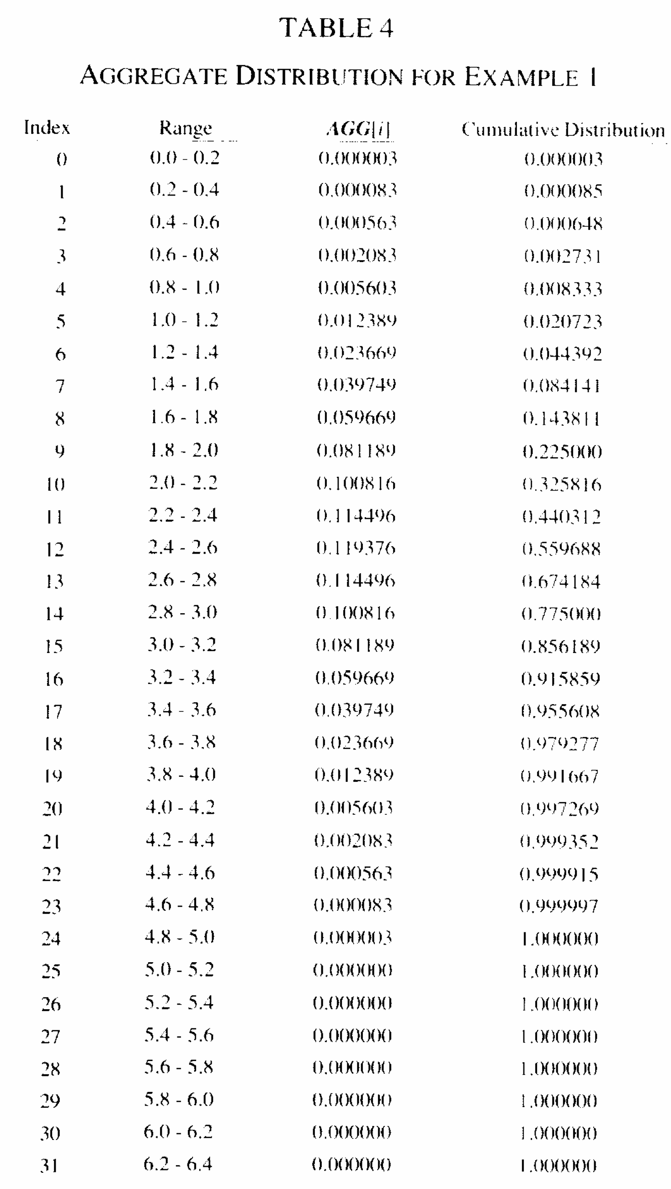
The consequence is that for a severity which is piecewise uniform, the algorithm is exact up to floating point. That is not true of a lattice method, and it makes Table 4 an unusual reproduction target: a published table with no discretization error in it at all.
aggregate is a lattice method. It does have a chistogram severity, a continuous histogram, and the technical guides note that a fine bucket size “approximates the continuous cdf approach” while recommending against it. This chapter is a check of that recommendation, and it ends up sharpening it.
2 Paper solution and gold standard
Section 4’s first example is deliberately minimal, “intended to be easy to reproduce in order to test an actual implementation. It is not meant to be realistic.” It computes the distribution of exactly five claims, each uniform on \([0,1]\). The grid is \(n = 32\) elements over \(L = 6.4\), so each element spans \(0.2\), and the severity vector is \((0.2, 0.2, 0.2, 0.2, 0.2, 0, \ldots, 0)\).
Since the sum of five variables each at most 1 cannot exceed 5, only the first 25 output elements are below 1. Table 4 lists all 32 cumulative values to six decimals.
The distribution of a sum of \(n\) independent standard uniforms is the Irwin-Hall law, with exact CDF
\[F_n(x) = \frac{1}{n!}\sum_{k=0}^{\lfloor x \rfloor} (-1)^k \binom{n}{k}(x-k)^n.\]
The paper checks itself against this: the sum of its first five elements is 0.008335, “which (up to rounding error) is \(1/120\)”. So the gold standard is not merely published, it is a closed form, and Table 4, Figure 1, should be \(F_5\) evaluated at multiples of \(0.2\). Table 1 checks that.
Figure 1: Robertson (1992), Table 4.
%xmode minimalfrom math import factorialimport numpy as npimport pandas as pdfrom scipy.special import combfrom bookstyle import GT, build, showdef irwin_hall(x, n=5):"""Exact CDF of a sum of n independent standard uniforms."""if x <=0:return0.0if x >= n:return1.0 k = np.arange(0, int(np.floor(x)) +1)returnfloat((((-1.0) ** k) * comb(n, k) * (x - k) ** n).sum() / factorial(n))# Values legible in the scan of Table 4. The scan is poor; these are the entries# that could be read without ambiguity.SCAN = {0.2: 0.000003, 1.0: 0.008333, 2.0: 0.225000, 2.6: 0.559688,3.6: 0.955608, 4.8: 0.999997, 5.0: 1.000000}GT(pd.DataFrame([{'x': x, 'Table 4 as scanned': v, 'Irwin-Hall exact': irwin_hall(x),'difference': v - irwin_hall(x)} for x, v in SCAN.items()] ).set_index('x'), formatters={'Table 4 as scanned': 6, 'Irwin-Hall exact': 6,'difference': '{x:.1e}'})
Exception reporting mode: Minimal
Table 1: The legible entries of Table 4 against the exact Irwin-Hall distribution function.
x
Table 4 as scanned
Irwin-Hall exact
difference
0.200
0.000003
0.000003
3.3e-07
1.000
0.008333
0.008333
-3.3e-07
2.000
0.225000
0.225000
0.0e+00
2.600
0.559688
0.559688
-1.1e-16
3.600
0.955608
0.955608
3.3e-16
4.800
0.999997
0.999997
-3.3e-07
5.000
1.000000
1.000000
0.0e+00
In Table 1 every legible entry agrees with the closed form to the six decimals printed, which confirms both the identification of the example and the claim that Robertson’s algorithm is exact here. The rest of this page therefore compares against irwin_hall rather than against the scan, which is the stronger comparison and does not depend on reading a 1992 photocopy.
EXACT = np.array([irwin_hall(k *0.2) for k inrange(1, 26)])F = s.density_df['F'].to_numpy()step =int(round(0.2/ s.bs))got = np.array([F[k * step] for k inrange(1, 26)])t4 = pd.DataFrame({'x': [round(k *0.2, 1) for k inrange(1, 26)],'exact': EXACT, 'aggregate': got}).set_index('x')t4['abs diff'] = (t4['aggregate'] - t4['exact']).abs()GT(t4, formatters={'exact': 8, 'aggregate': 8, 'abs diff': '{x:.2e}'})
Table 2: All 25 elements of Table 4 below the support cap, rebuilt on a lattice against the exact values.
x
exact
aggregate
abs diff
0.200
0.00000267
0.00000285
1.84e-07
0.400
0.00008533
0.00008814
2.80e-06
0.600
0.00064800
0.00066195
1.40e-05
0.800
0.00273067
0.00277441
4.37e-05
1.000
0.00833333
0.00843960
1.06e-04
1.200
0.02072267
0.02094137
2.19e-04
1.400
0.04439200
0.04478390
3.92e-04
1.600
0.08414133
0.08476279
6.21e-04
1.800
0.14381067
0.14469765
8.87e-04
2.000
0.22500000
0.22615207
1.15e-03
2.200
0.32581600
0.32718216
1.37e-03
2.400
0.44031200
0.44179535
1.48e-03
2.600
0.55968800
0.56116825
1.48e-03
2.800
0.67418400
0.67554146
1.36e-03
3.000
0.77500000
0.77613957
1.14e-03
3.200
0.85618933
0.85706268
8.73e-04
3.400
0.91585867
0.91646756
6.09e-04
3.600
0.95560800
0.95598980
3.82e-04
3.800
0.97927733
0.97948900
2.12e-04
4.000
0.99166667
0.99176876
1.02e-04
4.200
0.99726933
0.99731094
4.16e-05
4.400
0.99935200
0.99936505
1.31e-05
4.600
0.99991467
0.99991720
2.54e-06
4.800
0.99999733
0.99999748
1.51e-07
5.000
1.00000000
1.00000000
1.11e-15
GT(pd.DataFrame([{'elements compared': 25,'worst absolute difference': float(t4['abs diff'].max()),'at x': float(t4['abs diff'].idxmax()),'decimals printed in Table 4': 6,'reproduced to the printed precision': bool(t4['abs diff'].max() <5e-7),}]), formatters={'worst absolute difference': '{x:.2e}', 'at x': 1,'elements compared': 0, 'decimals printed in Table 4': 0})
Table 3: The worst error over Table 4, against the precision the paper prints.
elements compared
worst absolute difference
at x
decimals printed in Table 4
reproduced to the printed precision
25
1.48e-03
2.4
6
False
Table 2 and Table 3 are not a reproduction to the published precision. The worst absolute difference is \(1.5\times10^{-3}\), near the middle of the distribution, against a table printed to six decimals. The shape is right, the tails are right to five or six decimals, and the body is wrong in the third.
4 Comments
4.1 The error is O(h), which is why refinement will not rescue it
rows = []for d in (200, 400, 1000, 2000, 5000): a = build(CHIST, bs=1/ d, log2=int(np.ceil(np.log2(8* d)))) Fa = a.density_df['F'].to_numpy() st =int(round(0.2/ a.bs)) w =float(np.abs(np.array([Fa[k * st] for k inrange(1, 26)]) - EXACT).max()) rows.append({'bs': f'1/{d}', 'buckets per 0.2': st, 'worst abs error': w})conv = pd.DataFrame(rows)conv['ratio to previous'] = conv['worst abs error'].shift(1) / conv['worst abs error']conv['bs ratio to previous'] = [np.nan, 2, 2.5, 2, 2.5]GT(conv.set_index('bs'), formatters={'buckets per 0.2': 0, 'worst abs error': '{x:.3e}','ratio to previous': 3, 'bs ratio to previous': 1})
Table 4: Worst error over Table 4 as the bucket is refined, beside the refinement ratio, showing first order convergence.
bs
buckets per 0.2
worst abs error
ratio to previous
bs ratio to previous
1/200
40
1.483e-03
—
—
1/400
80
7.413e-04
2.001
2.0
1/1000
200
2.964e-04
2.501
2.5
1/2000
400
1.482e-04
2.000
2.0
1/5000
1,000
5.928e-05
2.500
2.5
In Table 4 the error ratio tracks the bandwidth ratio one for one: halve bs and the error halves. This is first order convergence, \(O(h)\), not the \(O(h^2)\) that Embrechts et al. (1993) establishes for a smooth severity. Reaching six decimals from \(1.5\times10^{-3}\) at first order needs about three thousand times the resolution, roughly bs = 1/600000, which is not a calculation anybody should run to match a 1992 table.
The reason for the lost order is the severity’s hard edges. A uniform density on \([0,1]\) is discontinuous at both ends, and the \(O(h^2)\) result needs a density with a uniformly continuous derivative. At a jump, a lattice cell straddles the discontinuity and the mass assigned to it is wrong at first order in \(h\), and no amount of grid refinement changes the order. Robertson’s method has no such term because it integrates the uniform pieces exactly, which is precisely the advantage the paper claims for it.
So the negative result is the informative one. On the one severity family where the piecewise uniform representation is exact, it beats a lattice method by an unbounded margin, and the example was chosen to be that family.
4.2 The chistogram adds nothing here, which is worth knowing
The technical guides suggest chistogram with a fine bs as a way to approximate the continuous approach. It is not: in Table 5 it is numerically the same as declaring the uniform severity directly and letting the default rounding discretize it.
UNIF ='agg Robertson2 5 claims sev 1 * uniform fixed'rows = []for label, prog, kw in [('chistogram, xps in five bins', CHIST, {}), ('plain uniform, sev_calc round', UNIF,dict(sev_calc='round')), ('plain uniform, sev_calc continuous', UNIF,dict(sev_calc='continuous')), ('plain uniform, sev_calc forward', UNIF,dict(sev_calc='forward')), ('plain uniform, sev_calc backward', UNIF,dict(sev_calc='backward'))]: a = build(prog, bs=1/200, log2=13, **kw) Fa = a.density_df['F'].to_numpy() st =int(round(0.2/ a.bs)) g = np.array([Fa[k * st] for k inrange(1, 26)]) rows.append({'route': label, 'worst abs error': float(np.abs(g - EXACT).max()),'F(2.0)': float(g[9])})GT(pd.DataFrame(rows).set_index('route'), formatters={'worst abs error': '{x:.6e}', 'F(2.0)': 8})
Table 5: Five routes to the same uniform severity, and the error each produces on Table 4.
route
worst abs error
F(2.0)
chistogram, xps in five bins
1.483352e-03
0.22615207
plain uniform, sev_calc round
1.483352e-03
0.22615207
plain uniform, sev_calc continuous
8.903602e-03
0.23192789
plain uniform, sev_calc forward
8.903602e-03
0.23192789
plain uniform, sev_calc backward
5.932631e-03
0.22043859
In Table 5 the chistogram row and the plain rounding row agree to every digit shown, including at \(F(2.0)\). Both are \(1.483\times10^{-3}\). So the elaborate route buys exactly nothing over sev 1 * uniform, and the two designs that actually try to be continuous, continuous and forward, are six times worse.
That sharpens the guides’ recommendation. Their stated reason for avoiding the approach is that it “is unnecessarily complicated and does not improve accuracy in any example we have encountered”. The measurement here says something stronger and more useful: on this example it does not merely fail to improve accuracy, it produces the identical numbers, so the complication is not a trade-off at any price.
4.3 What would be needed to reproduce it, and whether it is worth having
An exact reproduction of Table 4 needs the piecewise uniform severity carried analytically through the transform, which means the paper’s \(A'\) correction terms, not a finer lattice. That is a real feature and aggregate does not have it.
The case for adding it is weak, and Table 4 is the reason. The example was built so that the severity is exactly piecewise uniform, which is the one circumstance where the method is exact rather than merely better. A real claim size curve fitted by a step function is not exactly a step function, so the correction terms remove the discretization error of an approximation that was itself chosen for convenience. Against that, they cost roughly double the vector length, which the paper states. Given that Embrechts et al. (1993) recovers the missing order of accuracy for smooth severities by Richardson extrapolation at the cost of one extra build, and that hard-edged severities are rare in practice and easy to spot, the lattice route with refinement is the better default even though it loses this particular table.
This chapter is therefore a partial reproduction and is filed as one. The shape reproduces, the tails reproduce, the identification of the example is confirmed against a closed form, and the body misses the published precision by three orders of magnitude for a reason that is understood and structural rather than accidental.
Programs in the aggregate Loss Lab
Each program below opens in the aggregate Loss Lab, which builds it with nothing to install. The names are those in reproductions.agg, where every program is renamed by its paper’s citation key.
Embrechts, P., Grübel, R., & Pitts, S. M. (1993). Some applications of the fast Fourier transform algorithm in insurance mathematics. Statistica Neerlandica, 47(1), 59–75. https://doi.org/10.1111/j.1467-9574.1993.tb01406.x
Robertson, J. P. (1992). The computation of aggregate loss distributions. Proceedings of the Casualty Actuarial Society, 79(150), 57–133.
4 Comments
4.1 The error is O(h), which is why refinement will not rescue it
Table 4 refines the grid and watches the error.
In Table 4 the error ratio tracks the bandwidth ratio one for one: halve
bsand the error halves. This is first order convergence, \(O(h)\), not the \(O(h^2)\) that Embrechts et al. (1993) establishes for a smooth severity. Reaching six decimals from \(1.5\times10^{-3}\) at first order needs about three thousand times the resolution, roughlybs = 1/600000, which is not a calculation anybody should run to match a 1992 table.The reason for the lost order is the severity’s hard edges. A uniform density on \([0,1]\) is discontinuous at both ends, and the \(O(h^2)\) result needs a density with a uniformly continuous derivative. At a jump, a lattice cell straddles the discontinuity and the mass assigned to it is wrong at first order in \(h\), and no amount of grid refinement changes the order. Robertson’s method has no such term because it integrates the uniform pieces exactly, which is precisely the advantage the paper claims for it.
So the negative result is the informative one. On the one severity family where the piecewise uniform representation is exact, it beats a lattice method by an unbounded margin, and the example was chosen to be that family.
4.2 The chistogram adds nothing here, which is worth knowing
The technical guides suggest
chistogramwith a finebsas a way to approximate the continuous approach. It is not: in Table 5 it is numerically the same as declaring the uniform severity directly and letting the default rounding discretize it.In Table 5 the chistogram row and the plain rounding row agree to every digit shown, including at \(F(2.0)\). Both are \(1.483\times10^{-3}\). So the elaborate route buys exactly nothing over
sev 1 * uniform, and the two designs that actually try to be continuous,continuousandforward, are six times worse.That sharpens the guides’ recommendation. Their stated reason for avoiding the approach is that it “is unnecessarily complicated and does not improve accuracy in any example we have encountered”. The measurement here says something stronger and more useful: on this example it does not merely fail to improve accuracy, it produces the identical numbers, so the complication is not a trade-off at any price.
4.3 What would be needed to reproduce it, and whether it is worth having
An exact reproduction of Table 4 needs the piecewise uniform severity carried analytically through the transform, which means the paper’s \(A'\) correction terms, not a finer lattice. That is a real feature and
aggregatedoes not have it.The case for adding it is weak, and Table 4 is the reason. The example was built so that the severity is exactly piecewise uniform, which is the one circumstance where the method is exact rather than merely better. A real claim size curve fitted by a step function is not exactly a step function, so the correction terms remove the discretization error of an approximation that was itself chosen for convenience. Against that, they cost roughly double the vector length, which the paper states. Given that Embrechts et al. (1993) recovers the missing order of accuracy for smooth severities by Richardson extrapolation at the cost of one extra build, and that hard-edged severities are rare in practice and easy to spot, the lattice route with refinement is the better default even though it loses this particular table.
This chapter is therefore a partial reproduction and is filed as one. The shape reproduces, the tails reproduce, the identification of the example is confirmed against a closed form, and the body misses the published precision by three orders of magnitude for a reason that is understood and structural rather than accidental.