Grübel and Hermesmeier on aliasing and exponential tilting
Reproducing Grübel and Hermesmeier (1999)
Author
Stephen J. Mildenhall
Published
2026-10-22 19:56 commit b5ca906+
1 Context and problem
An FFT computes a circular convolution. Put a severity on a lattice of \(N\) buckets, transform, raise to the frequency’s probability generating function, invert, and any aggregate mass that should have landed beyond bucket \(N\) instead wraps around and lands in the low buckets. That is aliasing, and it is the one error in the transform approach that has nothing to do with discretization: it would be there even if the severity were exactly arithmetic.
Grübel and Hermesmeier (1999) is the paper that made this precise and gave the fix. Their Algorithm 1 is the unadorned transform method. Algorithm 5 adds exponential tilting: multiply the discretized severity by \(e^{-\theta k}\) before transforming and divide it back out afterwards. Tilting makes the sequence decay fast, so the mass that wraps is negligible before it wraps, and the aliasing error is suppressed by roughly \(e^{-\theta N}\). Their Theorem 2 bounds the total aliasing error by the mass of the untruncated aggregate at or beyond the truncation point.
The practical constraint is that \(\theta\) cannot be taken large: the untilting step multiplies by \(e^{+\theta k}\), and for \(k\) near \(N\) that is a huge factor which amplifies floating point noise. Their rule of thumb is \(\theta N \approx 20\).
aggregate does not tilt. It controls aliasing by padding, which doubles or quadruples the severity vector with zeros so there is nowhere for the wrap to go. Tilting is carried in aggregate.pedagogy for exactly this page’s purpose, as a teaching device rather than a production path, which makes the paper a test of a road the library deliberately did not take.
2 Paper solution and gold standard
Section 3 takes the claim size to be the stable law of index \(1/2\), following Embrechts et al. (1993). This is scipy.stats.levy, concentrated on the positive half line, and it has no mean. Frequency is Poisson with \(\lambda t = 20\). The lattice is \(N = 1024\) intervals of length 1, so the truncation point is \(x_0 = Nh = 1024\).
The index \(1/2\) is what makes an exact answer available. A stable law of index \(1/2\) satisfies \(f_\alpha \ast f_\beta = f_{\alpha+\beta}\) in the paper’s scale parameterization, so the \(n\)-fold convolution is another Lévy with a known scale, and the compound probability \(u([x - 0.5,\, x + 0.5])\) can be summed in closed form.
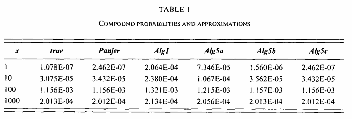
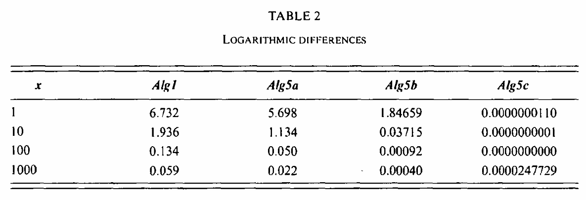
Table 1, Figure 1, gives six columns at \(x = 1, 10, 100, 1000\): the true value, the Panjer recursion on the same lattice, Algorithm 1, and Algorithm 5 at \(\theta N = 1, 5, 25\). Table 2, Figure 2, restates the last four as \(\log\) of the ratio to the Panjer value. The text adds two things neither table gives: the sum of absolute differences between Panjer and each transform algorithm over the whole lattice, and the value Theorem 2’s bound takes. Table 1 transcribes Table 1.
Table 1: Grübel and Hermesmeier (1999), Table 1 as printed.
x
true
Panjer
Alg1
Alg5a
Alg5b
Alg5c
1
1.078e-07
2.462e-07
0.0002064
7.346e-05
1.56e-06
2.462e-07
10
3.075e-05
3.432e-05
0.000238
0.0001067
3.562e-05
3.432e-05
100
0.001156
0.001156
0.001321
0.001215
0.001157
0.001156
1,000
0.0002013
0.0002012
0.0002134
0.0002056
0.0002013
0.0002012
3 The aggregate reproduction
The declaration is a one liner. levy takes no shape parameter, so the severity clause is bare.
a = build(f'agg Levy {LAM} claim sev levy poisson', update=False)a.update(log2=16, bs=BS, padding=2, normalize=False)show(a)
V:\worktrees\aggregate_REFACTOR\src\aggregate\_aggregate.py:4481: DefectiveDistributionWarning: Levy: aggregate PMF deficit 6.226e-02 (Σp = 1 − 6.226e-02 < 1); forwards and backwards S diverge by the deficit (forwards > backwards). Further occurrences this session are suppressed; each object records its own verdict in validation.
  rv = self.update_work(xs, debug=debug, x_min=x_min, x_max=x_max,
aggLevy20claimssevlevypoisson
The whole of Table 1 is assembled by one call, which computes the closed-form column from Lévy stability and sweeps the tilts, giving Table 2.
Table 2: Table 1 rebuilt, all six columns at the four tabulated points, beside the printed figures.
paper
aggregate
x
true
Panjer
Alg1
Alg5a
Alg5b
Alg5c
true
Panjer
Alg1
Alg5a
Alg5b
Alg5c
1
1.078e-07
2.462e-07
0.0002064
7.346e-05
1.56e-06
2.462e-07
1.078e-07
2.462e-07
0.0002064
7.346e-05
1.56e-06
2.462e-07
10
3.075e-05
3.432e-05
0.000238
0.0001067
3.562e-05
3.432e-05
3.075e-05
3.432e-05
0.000238
0.0001067
3.562e-05
3.432e-05
100
0.001156
0.001156
0.001321
0.001215
0.001157
0.001156
0.001155
0.001156
0.001321
0.001215
0.001157
0.001156
1,000
0.0002013
0.0002012
0.0002134
0.0002056
0.0002013
0.0002012
0.0002013
0.0002012
0.0002134
0.0002056
0.0002013
0.0002012
rel = (got / TABLE1 -1).abs()GT(pd.DataFrame([{'column': c, 'worst relative difference': float(rel[c].max())}for c in TABLE1.columns]).set_index('column'), formatters={'worst relative difference': '{x:.1e}'})
Table 3: Worst relative difference from Table 1, column by column.
column
worst relative difference
true
4.5e-04
Panjer
1.6e-04
Alg1
2.3e-04
Alg5a
1.8e-04
Alg5b
1.2e-04
Alg5c
1.6e-04
By Table 3 every one of the 24 published values comes back inside the four significant figures printed. Table 2 restates four of those columns as logarithms of ratios, which is a sharper test in the small columns because it removes the shared scale, in Table 4.
Table 4: Table 2 rebuilt, each algorithm as the log of its ratio to the Panjer value, beside the printed figures.
paper
aggregate
x
Alg1
Alg5a
Alg5b
Alg5c
Alg1
Alg5a
Alg5b
Alg5c
1
6.732000
5.698000
1.846590
0.000000
6.731818
5.698487
1.846586
0.000000
10
1.936000
1.134000
0.037150
0.000000
1.936384
1.133992
0.037151
0.000000
100
0.134000
0.050000
0.000920
0.000000
0.133675
0.049719
0.000917
0.000000
1,000
0.059000
0.022000
0.000400
0.000025
0.058864
0.021650
0.000396
-0.000016
3.1 The two numbers that are not in a table
The text reports the sum of absolute differences between Panjer and each transform algorithm, over the whole lattice rather than the four tabulated points. That is a much stronger check than any single row, since it uses all 1024 buckets. Table 5 is the comparison.
ref = a.density_df.p_total.to_numpy()[:N].copy() # padded, so unaliasedrows = []for tilt, paper inzip(TILTS, L1_PAPER): v = tilted_aggregate_density(a, log2=10, bs=BS, padding=0, tilt=tilt).to_numpy()[:N] name ='Alg1 (no tilt)'if tilt isNoneelsef'Alg5, theta N = {tilt * N:.0f}' rows.append({'algorithm': name, 'paper': paper,'aggregate': float(np.abs(ref - v).sum())})l1 = pd.DataFrame(rows).set_index('algorithm')l1['ratio'] = l1['aggregate'] / l1['paper']GT(l1, formatters={'paper': '{x:.4g}', 'aggregate': '{x:.4g}', 'ratio': 3})
Table 5: Sum of absolute differences from the unaliased density over the whole lattice, for each algorithm.
algorithm
paper
aggregate
ratio
Alg1 (no tilt)
0.0714
0.07138
1.000
Alg5, theta N = 1
0.0255
0.0255
1.000
Alg5, theta N = 5
0.000459
0.0004592
1.001
Alg5, theta N = 25
3.121e-07
2.013e-07
0.645
In Table 5 three of the four match to the printed precision: 0.07138 against 0.0714, 0.02550 against 0.0255, and 0.00045924 against 0.000459. The fourth does not, and the paper says why before it is asked. At \(\theta N = 25\) the untilting step multiplies by factors “of the order \(10^{10}\)” and “rounding errors begin to be important”. Both values are at the \(10^{-7}\) level, four orders of magnitude below the next one up, so the comparison there is between two different floating point noise floors rather than between two algorithms.
Theorem 2 bounds the aliasing error by the mass of the untruncated aggregate at or beyond the truncation point, which is exactly the survival function at \(x_0\), evaluated in Table 6.
# `tilted_aggregate_density` updates the object it is handed, so `a` is sitting# on the coarse log2=10 grid after the sweep above. Put it back first.a.update(log2=16, bs=BS, padding=2, normalize=False)p = a.density_df.p_total.to_numpy()GT(pd.DataFrame([ {'quantity': 'mass on the 2^16 grid', 'value': float(p.sum())}, {'quantity': 'deficit above the grid', 'value': 1-float(p.sum())}, {'quantity': 'mass in buckets [1024, grid end)', 'value': float(p[N:].sum())}, {'quantity': 'total at or beyond 1024, the Theorem 2 bound','value': float(p[N:].sum()) +1-float(p.sum())}, {'quantity': 'S(1023) read off density_df','value': float(a.density_df.S.loc[N -1])}, {'quantity': 'paper', 'value': THEOREM2_PAPER},]).set_index('quantity'), float_format=6)
Table 6: The Theorem 2 bound assembled from the on-grid tail and the mass above the grid, against the paper’s 0.4641.
quantity
value
mass on the 2^16 grid
0.937738
deficit above the grid
0.062262
mass in buckets [1024, grid end)
0.401806
total at or beyond 1024, the Theorem 2 bound
0.464068
S(1023) read off density_df
0.464068
paper
0.464100
Table 6 gives 0.4641, to the four figures printed. Getting there needs one thing said out loud: the severity has no mean, so at bs = 1 even a \(2^{16}\) grid carries only 93.8% of the aggregate, and the 6.2% above it is part of the bound. Summing the on-grid tail alone gives 0.4018 and misses.
4 Comments
4.1 The bound is loose, and the paper knows why
The actual aliasing error in Table 5 is 0.0714 against the 0.4641 bound of Table 6, a factor of 6.5. The paper attributes this to the claim size being subexponential, and it is the right diagnosis: for a subexponential severity the aggregate tail is dominated by the single largest claim, so the mass beyond the truncation point is concentrated far beyond it, and wrapping mass that lands at \(x + 1024\) for large \(x\) mostly re-wraps out of the low buckets rather than into them. A bound that counts every unit of escaping mass as a unit of contamination cannot see that.
The practical consequence is that Theorem 2 is a certificate rather than a diagnostic. It tells you when you are definitely safe. It does not tell you how much error you actually have, and for a heavy tail it will talk you into a finer grid than you need.
4.2 The discretization error is the larger of the two, and it is the other paper
The paper’s closing observation about Table 1 is easy to miss and is the most interesting thing in it: “a comparison of the values in the second and third column of Table 1 shows that there is a pronounced discretization error, again most notable for small \(x\)-values.”
Table 7: The true value against the Panjer value on the same lattice, isolating discretization error from aliasing.
x
true
Panjer
Panjer / true
1
1.078e-07
2.462e-07
2.2839
10
3.075e-05
3.432e-05
1.1161
100
0.001156
0.001156
1.0000
1,000
0.0002013
0.0002012
0.9995
In Table 7, at \(x = 1\) the recursion on a lattice of span 1 is wrong by a factor of 2.3, and no amount of tilting or padding touches it, because both columns use the same discretized severity. Tilting fixes aliasing, and Table 1’s own second and third columns show that aliasing was not the binding constraint at the left hand end. That is the subject of Part II, Grübel and Hermesmeier (2000), and the same distinction is why aggregate reports discretization and aliasing as separate diagnostics rather than one error budget.
4.3 Why the library pads instead
Padding and tilting solve the same problem, and the reproduction shows they solve it about equally well: the paper’s own \(\theta N = 25\) column and the padded column agree to four figures at every \(x\). Padding wins on two counts that only show up in production.
It has no free parameter. The tilt has to be chosen, the good range is bounded below by the aliasing it has to kill and above by the floating point amplification in the untilting step, and the paper’s own \(\theta N \approx 20\) rule is a compromise between two failure modes. Padding has one setting, “how much”, and more is monotonically safer.
And it does not amplify. The fourth row of Table 5 is the whole argument: at the tilt the paper recommends, the answer is already limited by rounding noise introduced by the method itself rather than by the aliasing it removed. A doubling of the vector length costs one factor of two in the transform and introduces nothing.
Programs in the aggregate Loss Lab
Each program below opens in the aggregate Loss Lab, which builds it with nothing to install. The names are those in reproductions.agg, where every program is renamed by its paper’s citation key.
Grubel1999.Levy: a compound Poisson Levy severity, the aliasing case tilting repairs.
Embrechts, P., Grübel, R., & Pitts, S. M. (1993). Some applications of the fast Fourier transform algorithm in insurance mathematics. Statistica Neerlandica, 47(1), 59–75. https://doi.org/10.1111/j.1467-9574.1993.tb01406.x
Grübel, R., & Hermesmeier, R. (1999). Computation of Compound Distributions I: Aliasing Errors and Exponential Tilting. Astin Bulletin, 29(2), 197–214. https://doi.org/10.2143/AST.29.2.504611
Grübel, R., & Hermesmeier, R. (2000). Computation of Compound Distributions II: Discretization Errors and Richardson Extrapolation. ASTIN Bulletin, 30(2), 309–332. https://doi.org/10.2143/AST.30.2.504638
4 Comments
4.1 The bound is loose, and the paper knows why
The actual aliasing error in Table 5 is 0.0714 against the 0.4641 bound of Table 6, a factor of 6.5. The paper attributes this to the claim size being subexponential, and it is the right diagnosis: for a subexponential severity the aggregate tail is dominated by the single largest claim, so the mass beyond the truncation point is concentrated far beyond it, and wrapping mass that lands at \(x + 1024\) for large \(x\) mostly re-wraps out of the low buckets rather than into them. A bound that counts every unit of escaping mass as a unit of contamination cannot see that.
The practical consequence is that Theorem 2 is a certificate rather than a diagnostic. It tells you when you are definitely safe. It does not tell you how much error you actually have, and for a heavy tail it will talk you into a finer grid than you need.
4.2 The discretization error is the larger of the two, and it is the other paper
The paper’s closing observation about Table 1 is easy to miss and is the most interesting thing in it: “a comparison of the values in the second and third column of Table 1 shows that there is a pronounced discretization error, again most notable for small \(x\)-values.”
In Table 7, at \(x = 1\) the recursion on a lattice of span 1 is wrong by a factor of 2.3, and no amount of tilting or padding touches it, because both columns use the same discretized severity. Tilting fixes aliasing, and Table 1’s own second and third columns show that aliasing was not the binding constraint at the left hand end. That is the subject of Part II, Grübel and Hermesmeier (2000), and the same distinction is why
aggregatereports discretization and aliasing as separate diagnostics rather than one error budget.4.3 Why the library pads instead
Padding and tilting solve the same problem, and the reproduction shows they solve it about equally well: the paper’s own \(\theta N = 25\) column and the padded column agree to four figures at every \(x\). Padding wins on two counts that only show up in production.
It has no free parameter. The tilt has to be chosen, the good range is bounded below by the aliasing it has to kill and above by the floating point amplification in the untilting step, and the paper’s own \(\theta N \approx 20\) rule is a compromise between two failure modes. Padding has one setting, “how much”, and more is monotonically safer.
And it does not amplify. The fourth row of Table 5 is the whole argument: at the tilt the paper recommends, the answer is already limited by rounding noise introduced by the method itself rather than by the aliasing it removed. A doubling of the vector length costs one factor of two in the transform and introduces nothing.