Embrechts and Frei (2009) is a head to head comparison: Panjer recursion against FFT for compound distributions. Both need the continuous severity replaced by a lattice distribution \(F_h\) of bandwidth \(h\), and the paper’s most useful section is about that step rather than about either transform.
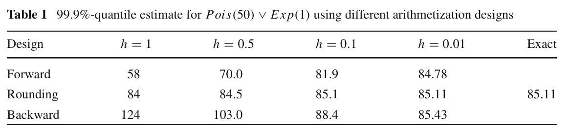
There are three natural ways to discretize. Forward puts each cell’s mass at its lower endpoint, backward at its upper endpoint, and rounding splits it so the cell’s mean survives. The first two are the classical bounds: forward makes every claim smaller so it understates the aggregate, backward overstates it, and the true answer is between them. Rounding is not a bound at all, and that is the point of the paper’s Table 1.
The paper also treats aliasing, recommending tilting where the interest is in the body of the distribution and noting that padding as in Wang (1998) does the same job. aggregate takes the padding branch, and its rounding default is the design Table 1 identifies as the accurate one, so this is a reproduction of the reasoning behind two library defaults.
2 Paper solution and gold standard
Table 1, Figure 1, estimates the 99.9% quantile of \(\mathrm{Pois}(50)\vee\mathrm{Exp}(1)\) at four bandwidths under all three designs, with an exact column. Table 1 transcribes it.
Table 2: The 99.9% quantile from the closed form series, against the paper’s exact column.
quantity
value
99.9% quantile from the closed-form series
85.105955
paper, Exact column
85.110000
E[S] exact
50.000000
Table 2 gives 85.10596, which is 85.11 to the two decimals printed. The gold standard is sound before anything is convolved.
3 The aggregate reproduction
sev_calc selects the design, so all three of the paper’s rows are one keyword apart. The grid is sized to reach 400, comfortably past the quantile of interest, at every bandwidth.
def ef(h, design): log2 =int(np.ceil(np.log2(400/ h)))return build('agg EF 50 claims sev expon poisson', bs=h, log2=log2, padding=1, sev_calc=design, normalize=False)show(ef(0.01, 'round'))rows = []for design, label in [('forward', 'forward'), ('round', 'rounding'), ('backward', 'backward')]: rows.append({'design': label,**{f'h = {h:g}': ef(h, design).q(0.999)for h in (1.0, 0.5, 0.1, 0.01)}})got = pd.DataFrame(rows).set_index('design')GT(pd.concat({'paper': PAPER, 'aggregate': got}, axis=1), float_format=2)
Table 3: Table 1 rebuilt, the 99.9% quantile under all three designs at four bandwidths, beside the printed figures.
Table 4: Worst absolute difference from Table 1, design by design.
design
worst absolute difference
forward
0.000
rounding
0.000
backward
0.000
all twelve
0.000
In Table 3 and Table 4 all twelve values reproduce exactly, to every digit printed, across three designs and four bandwidths. That is the strongest form this comparison can take: the paper’s table is not being approximated, it is being recovered.
3.1 What the table is actually saying
The numbers matter less than their arrangement, and the arrangement is easy to miss in a small table. Table 5 sets it out.
rows = []for h in (1.0, 0.5, 0.1, 0.01): f, r, b = (got.loc[d, f'h = {h:g}'] for d in ('forward', 'rounding', 'backward')) rows.append({'h': h, 'bracket width, backward minus forward': b - f,'rounding error': r - q_exact,'forward error': f - q_exact, 'backward error': b - q_exact})GT(pd.DataFrame(rows).set_index('h'), float_format=3)
Table 5: The width of the forward to backward bracket at each bandwidth, beside the error of each design.
h
bracket width, backward minus forward
rounding error
forward error
backward error
1.000
66.000
-1.11e+00
-2.71e+01
3.89e+01
0.500
33.000
-6.06e-01
-1.51e+01
1.79e+01
0.100
6.500
-5.96e-03
-3.21e+00
3.29e+00
0.010
0.650
4.04e-03
-3.26e-01
3.24e-01
In Table 5, at \(h = 1\) the bounds are 58 and 124, a bracket 66 wide around a true value of 85.1, which is useless for any practical purpose. Rounding at the same bandwidth gives 84, an error of 1.1. The bounds do bracket, honestly and always, and they do it so loosely that at any bandwidth a practitioner would actually use, the bracket is worth less than the point estimate it contains.
That is why aggregate has a rounding default and no bounds mode. It is the same conclusion Gerber (1982) reached from the other end, in 1982, with the same ranking of the same three methods.
The cost of the default is that it is not conservative in any direction. Rounding is a better estimate and a worse guarantee, and the honest error control is refinement: rounding at \(h = 1\), \(0.5\), \(0.1\) gives 84, 84.5, 85.1, which converges visibly on its own without needing the bounds to confirm it.
4 Figure 1: the Poisson/Pareto aliasing picture
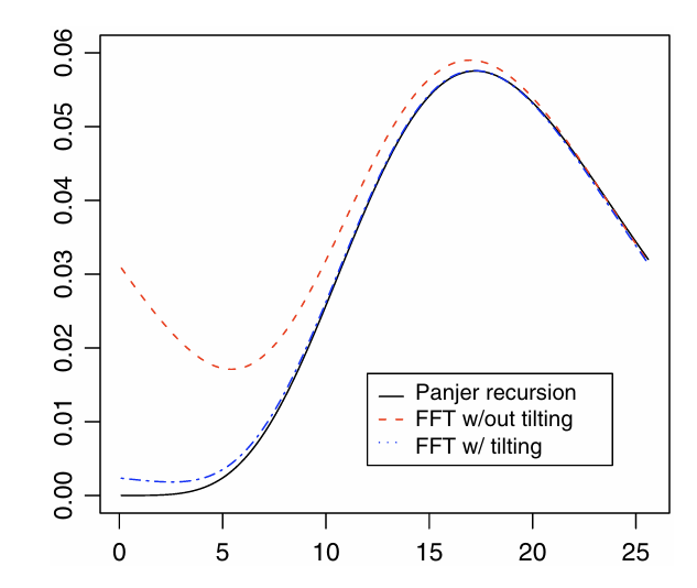
Section 3 illustrates aliasing on \(\mathrm{Pois}(20)\vee\mathrm{Pareto}(4, 3)\), a severity with finite mean and infinite third moment. There is no published table for Figure 2, so the reproduction is of the shape and the regime change rather than of numbers.
Figure 2: Approximate densities for \(Pois(20)\vee Pareto(4,3)\), Embrechts and Frei (2009), Figure 1.
V:\worktrees\aggregate_REFACTOR\src\aggregate\_bucket_window.py:1430: InfeasibleGridWarning: EF1: severity 'pareto' cannot be reproduced on this grid. The body needs bs <= 0.0174043 (0.2431% of the mean is supplied below the first half bucket, and is placed at 0); the mean is not complete until the grid reaches 125.507, so matching it to 0.0001 needs log2 = 13, and log2 = 8 was used. A thick unlimited severity has this problem at any bucket size, because its mean is furnished far above its median and a finer bs only shortens the reach. Add an occurrence limit, or accept the reported moment errors. Further occurrences this session are suppressed; each object records its own verdict in validation.
  warn_infeasible_grid(agg)
V:\worktrees\aggregate_REFACTOR\src\aggregate\_aggregate.py:4481: DefectiveDistributionWarning: EF1: aggregate PMF deficit 1.087e-03 (Σp = 1 − 1.087e-03 < 1); forwards and backwards S diverge by the deficit (forwards > backwards). Further occurrences this session are suppressed; each object records its own verdict in validation.
  rv = self.update_work(xs, debug=debug, x_min=x_min, x_max=x_max,
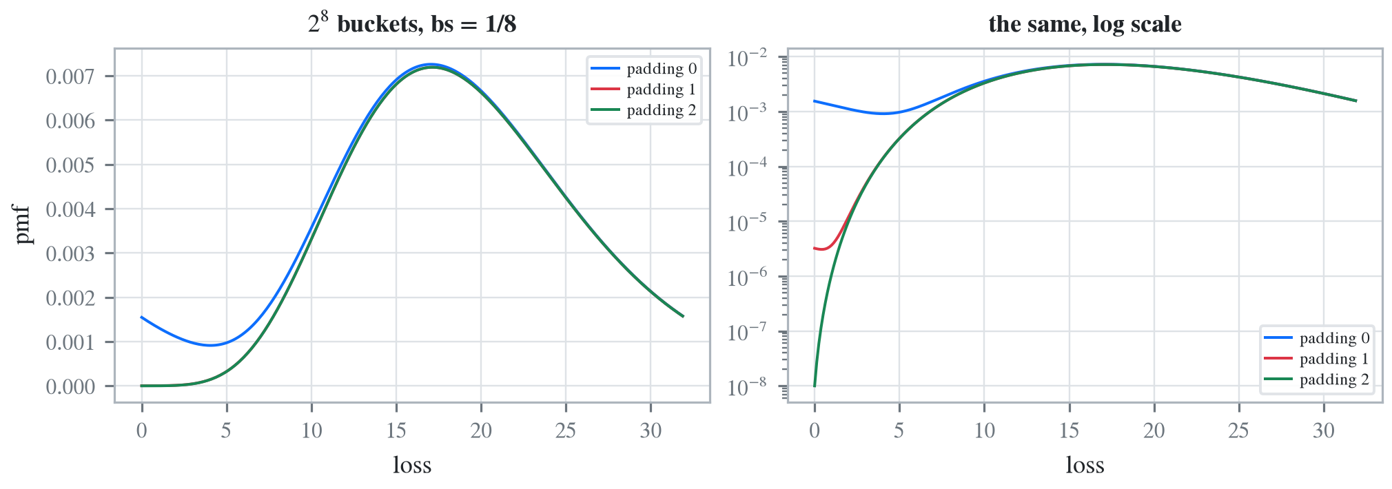
Figure 3: Reproducing Figure 1. The aggregate density at three padding levels, on a linear and a log scale.
In Figure 3 the untilted, unpadded curve turns up at the right hand end, which is aliased mass that belongs beyond the grid, and the log panel shows padding removing it completely. The paper’s point that padding and tilting are equally effective is the same finding Grübel and Hermesmeier (1999) arrives at from the tilting side and Schaller and Temnov (2008) from the operational risk side, and this page’s Table 1 result is why the library only needs one of them.
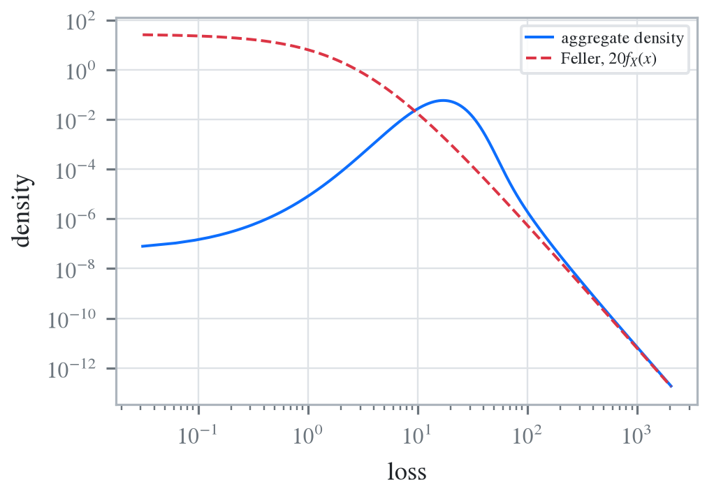
Figure 4: The far tail against Feller’s asymptotic, twenty times the severity survival function.
Differentiating Feller’s theorem gives the aggregate density approaching \(\lambda f_X(x)\) in the far tail, and in Figure 4 the two curves meet once the Poisson body is left behind. The change of regime, from a body dominated by the claim count to a tail dominated by the single largest claim, is visible as the kink.
5 Comments
5.1 The three designs are still there, and one is missing on purpose
aggregate implements forward, backward and round, so all three of Table 1’s rows are reachable, and the moment design that would preserve two moments raises NotImplementedError. The paper’s table is the argument for that gap: since rounding already beats both bounds by an order of magnitude at every bandwidth, a fourth design has to justify itself against rounding rather than against the bounds, and none of the candidates does.
5.2 Where the bounds do earn their keep
The bracket is useless as an error bar and valuable as a test. If a build’s forward and backward estimates do not straddle its rounding estimate, something is wrong with the grid rather than with the discretization: the most likely cause is that aliasing or truncation is larger than the discretization error, so the three designs are all being dominated by an error that has nothing to do with the design. Table 6 runs that test on an adequate grid and on a short one.
rows = []for h, pad in [(0.5, 1), (0.5, 0)]: vals = {}for design, label in [('forward', 'forward'), ('round', 'rounding'), ('backward', 'backward')]: log2 =6if pad ==0elseint(np.ceil(np.log2(400/ h))) b = build('agg EF 50 claims sev expon poisson', bs=h, log2=log2, padding=pad, sev_calc=design, normalize=False) vals[label] = b.q(0.999) rows.append({'h': h, 'log2': log2, 'padding': pad, **vals,'brackets': bool(vals['forward'] <= vals['rounding']<= vals['backward'])})GT(pd.DataFrame(rows).set_index(['h', 'log2', 'padding']), float_format=2)
V:\worktrees\aggregate_REFACTOR\src\aggregate\_bucket_window.py:1430: InfeasibleGridWarning: EF: severity 'expon' cannot be reproduced on this grid. The body needs bs <= 0.020067 (2.65% of the mean is supplied below the first half bucket, and is placed at 0); the mean is not complete until the grid reaches 12.5067, so matching it to 0.0001 needs log2 = 9, and log2 = 6 was used. A thick unlimited severity has this problem at any bucket size, because its mean is furnished far above its median and a finer bs only shortens the reach. Add an occurrence limit, or accept the reported moment errors. Further occurrences this session are suppressed; each object records its own verdict in validation.
  warn_infeasible_grid(agg)
Table 6: The three designs on an adequate grid and on one too short, showing where the bracket ordering fails.
h
log2
padding
forward
rounding
backward
brackets
0.50
10
1
70.00
84.50
103.00
True
6
0
31.50
31.50
31.50
True
In Table 6 the ordering holds on an adequate grid. On a grid too short to hold the distribution it fails, and the failure is informative in a way the individual numbers are not: it says the bandwidth is no longer the binding constraint. That is worth more than a bound, and it costs two extra builds.
Programs in the aggregate Loss Lab
Each program below opens in the aggregate Loss Lab, which builds it with nothing to install. The names are those in reproductions.agg, where every program is renamed by its paper’s citation key.
Embrechts2009a.EF: the compound Poisson exponential compared across three designs.
Embrechts2009a.EF1: the compound Poisson Pareto compared across the same three.
Embrechts, P., & Frei, M. (2009). Panjer recursion versus FFT for compound distributions. Mathematical Methods of Operations Research, 69(3), 497–508. https://doi.org/10.1007/s00186-008-0249-2
Gerber, H. U. (1982). On the numerical evaluation of the distribution of aggregate claims and its stop-loss premiums. Insurance Mathematics and Economics, 1(1), 13–18. https://doi.org/10.1016/0167-6687(82)90016-6
Grübel, R., & Hermesmeier, R. (1999). Computation of Compound Distributions I: Aliasing Errors and Exponential Tilting. Astin Bulletin, 29(2), 197–214. https://doi.org/10.2143/AST.29.2.504611
Schaller, P., & Temnov, G. (2008). Efficient and Precise Computation of Convolutions: Applying FFTs to Heavy Tailed Distributions. Computational Methods in Applied Mathematics, 8(2), 187–200.
5 Comments
5.1 The three designs are still there, and one is missing on purpose
aggregateimplementsforward,backwardandround, so all three of Table 1’s rows are reachable, and themomentdesign that would preserve two moments raisesNotImplementedError. The paper’s table is the argument for that gap: since rounding already beats both bounds by an order of magnitude at every bandwidth, a fourth design has to justify itself against rounding rather than against the bounds, and none of the candidates does.5.2 Where the bounds do earn their keep
The bracket is useless as an error bar and valuable as a test. If a build’s forward and backward estimates do not straddle its rounding estimate, something is wrong with the grid rather than with the discretization: the most likely cause is that aliasing or truncation is larger than the discretization error, so the three designs are all being dominated by an error that has nothing to do with the design. Table 6 runs that test on an adequate grid and on a short one.
In Table 6 the ordering holds on an adequate grid. On a grid too short to hold the distribution it fails, and the failure is informative in a way the individual numbers are not: it says the bandwidth is no longer the binding constraint. That is worth more than a bound, and it costs two extra builds.