Denuit (2019) connects the conditional mean risk sharing rule to the size-biased transform. The rule allocates \(\kappa_i(s) = \mathsf E[X_i \mid S = s]\) to participant \(i\); the paper’s representation formula rewrites that conditional expectation in terms of the size-biased version \(\widetilde{X}_i\), whose density is \(x f_i(x)/\mathsf E[X_i]\), and then reads off closed forms for compound Poisson and compound negative binomial pools.
The practical payoff is a result the paper uses in its own example and which is worth stating on its own: if two participants have the same claim severity distribution, then their combined share of any total loss \(s\) is the ratio of their combined expected claim frequency to the pool’s, independent of \(s\). Pooling participants with a common severity collapses to pooling frequencies.
That statement is an exact invariant, which makes this a reproduction with something firmer than a figure to check against.
2 Paper solution and gold standard
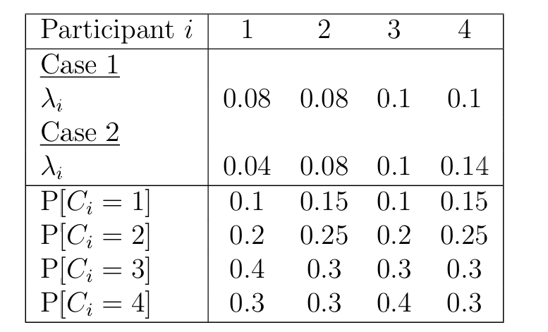
Section 6.1 describes a four participant peer to peer pool. Severities take values in \(\{1,2,3,4\}\), frequencies are Poisson, and case 1 sets \(\lambda = (0.08, 0.08, 0.10, 0.10)\).
The paper publishes three things this page can check:
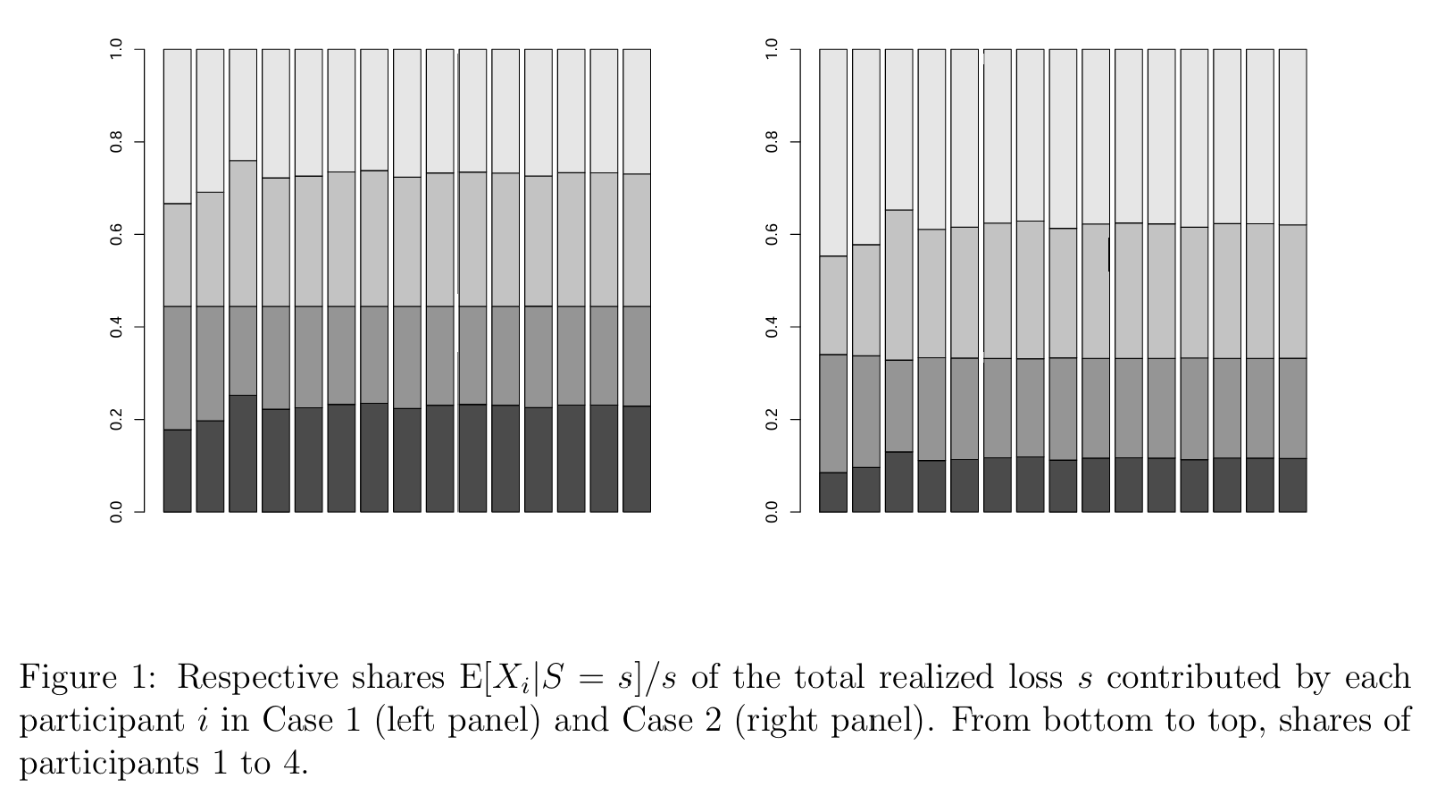
that Figure 1 shows “an horizontal line … separating the shares of participants 1-2 from the share of participants 3-4”, because participants 1 and 3 share a severity distribution and so do 2 and 4, so 1 and 2 together always contribute \((\lambda_1 + \lambda_2)/\lambda_\bullet\).
2.1 A discrepancy that has to be resolved first
Figure 1 and the paper’s text disagree about participant 3. The text says plainly that “Participants 1 and 3 have identical severity distributions, as well as participants 2 and 4”, which makes participant 3’s severity \((0.1, 0.2, 0.4, 0.3)\), the same as participant 1’s. The column for participant 3, as I read it, prints \((0.1, 0.2, 0.3, 0.4)\), with the last two entries swapped.
Only one of those can produce the horizontal line, so the paper’s own Figure 1 decides it. Figure 1 is the table in question and Table 1 tests the two readings.
Figure 1: Denuit (2019), Section 6.1, the pool.
%xmode minimalimport numpy as npimport pandas as pdimport matplotlib.pyplot as pltfrom aggregate.constants import FIG_W, FIG_Hfrom bookstyle import GT, build, showLAM = [0.08, 0.08, 0.10, 0.10]SEV_A ='[.1 .2 .4 .3]'# participant 1, and participant 3 per the textSEV_B ='[.15 .25 .3 .3]'# participants 2 and 4SEV_TABLE3 ='[.1 .2 .3 .4]'# participant 3 as the table column readsPAPER_S1 = [0.178, 0.267, 0.222, 0.333]def pool(sev3, name='Denuit61'):return build(f'''port {name} agg P1 {LAM[0]} claims dsev [1 2 3 4] {SEV_A} poisson agg P2 {LAM[1]} claims dsev [1 2 3 4] {SEV_B} poisson agg P3 {LAM[2]} claims dsev [1 2 3 4] {sev3} poisson agg P4 {LAM[3]} claims dsev [1 2 3 4] {SEV_B} poisson''', bs=1, log2=10)rows = []for label, sev3, nm in [('text: participant 3 matches participant 1', SEV_A, 'D61a'), ('table column 3 as printed', SEV_TABLE3, 'D61b')]: p = pool(sev3, nm) d = p.density_df share12 = np.array([float(d.loc[s, 'exeqa_P1'] + d.loc[s, 'exeqa_P2']) / sfor s inrange(1, 16)]) rows.append({'reading': label,'participants 1+2 share, min over s = 1..15': share12.min(),'max': share12.max(),'constant to 1e-9': bool(np.ptp(share12) <1e-9)})GT(pd.DataFrame(rows).set_index('reading'), float_format=6)
Exception reporting mode: Minimal
Table 1: The combined share of participants 1 and 2 over \(s = 1\) to \(15\), under each reading of participant 3’s severity.
reading
participants 1+2 share, min over s = 1..15
max
constant to 1e-9
text: participant 3 matches participant 1
0.444444
0.444444
True
table column 3 as printed
0.410518
0.481587
False
In Table 1 the text’s reading gives a share for participants 1 and 2 that is constant to machine precision over the whole plotted range. The table’s reading wanders between 0.41 and 0.48 and has no horizontal line anywhere. Figure 1 shows a horizontal line, so the text is right and the table’s third column is wrong, and the rest of this page uses the text.
Whether the fault is in the published table or in my scan of it I cannot tell, so this is recorded as a discrepancy rather than as an erratum.
3 The aggregate reproduction
Each participant is one agg with a Poisson frequency and a four point discrete severity. \(\kappa_i\) is the exeqa_ column, so no allocation code is needed. Table 2 checks the pool against three known values before any share is read.
p = pool(SEV_A)show(p)
port Denuit61agg P10.08claimsdsev[1234][0.10.20.40.3]poissonagg P20.08claimsdsev[1234][0.150.250.30.3]poissonagg P30.1claimsdsev[1234][0.10.20.40.3]poissonagg P40.1claimsdsev[1234][0.150.250.30.3]poisson
Table 2: The pool mean, the 99.9% quantile and the invariant group share, each against its exact value.
quantity
value
exact
E[S] from the pool
1.017000
1.017000
99.9% quantile of S
11.000000
11.000000
(lam1 + lam2) / lam total
0.444444
0.444444
got = [float(d.loc[1, f'exeqa_P{i}']) for i in (1, 2, 3, 4)]GT(pd.DataFrame({'participant': [1, 2, 3, 4], 'aggregate share at s = 1': got,'paper': PAPER_S1,'difference': [g - q for g, q inzip(got, PAPER_S1)]} ).set_index('participant'), formatters={'aggregate share at s = 1': 6, 'paper': 3,# sugar has no sign flag; `formatters` accepts a callable'difference': lambda x: f'{x:+.5f}'})
Table 3: The four shares at \(s = 1\), against the values the paper publishes.
participant
aggregate share at s = 1
paper
difference
1
0.177778
0.178
-0.00022
2
0.266667
0.267
-0.00033
3
0.222222
0.222
+0.00022
4
0.333333
0.333
+0.00033
In Table 3 all four published shares reproduce to within 0.0003, which is the paper’s rounding to three decimals: 0.17778 against 0.178, 0.26667 against 0.267, 0.22222 against 0.222, 0.33333 against 0.333. The 99.9% quantile is 11 as stated.
The paper derives those four numbers by hand, from the observation that \(S = 1\) implies exactly one claim of size 1, so the shares are the relative probabilities of that claim belonging to each participant. That gives \(\lambda_i \Pr[C_i = 1]\) normalized, which is a check that needs no software at all, in Table 4.
ss = np.arange(1, 16)sh = pd.DataFrame( {f'participant {i}': [float(d.loc[s, f'exeqa_P{i}']) / s for s in ss]for i in (1, 2, 3, 4)}, index=ss)fig, axs = plt.subplots(1, 2, figsize=(2* FIG_W, FIG_H), layout='constrained')sh.plot(ax=axs[0], lw=1, marker='.', ms=3)axs[0].set(xlabel='s', ylabel='share of s', title='individual shares', ylim=(0, 0.5))axs[0].legend(fontsize=6)(sh['participant 1'] + sh['participant 2']).plot( ax=axs[1], lw=1, marker='.', ms=3, label='participants 1 + 2')(sh['participant 3'] + sh['participant 4']).plot( ax=axs[1], lw=1, marker='.', ms=3, label='participants 3 + 4')for y in (sum(LAM[:2]) /sum(LAM), sum(LAM[2:]) /sum(LAM)): axs[1].axhline(y, ls='--', lw=0.6, c='C7')axs[1].set(xlabel='s', ylabel='share of s', title='the horizontal separation', ylim=(0, 1))axs[1].legend(fontsize=6)
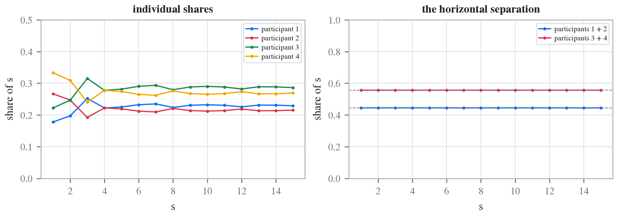
Figure 3: Reproducing Figure 1. Share of the total loss contributed by each participant, and the horizontal separation at 4/9.
The left panel of Figure 3 is the paper’s figure: four irregular curves, the irregularity coming from the discreteness of the severities, with participant 1 below participant 2 throughout because its severity is the lighter of the two. The right panel is the invariant, and the two group shares sit exactly on \(4/9\) and \(5/9\) at every \(s\) while the individual shares inside them move.
4 Comments
4.1 The invariant is the reproduction
The four numbers at \(s = 1\) are a good check and a weak one: they are determined by a single event, one claim of size one, and the paper computes them by hand precisely because that case is elementary. Any implementation that got the frequencies and the first severity probability right would match them.
The horizontal line is the strong check, and it is strong for a structural reason. It holds at every \(s\) simultaneously, it depends on the whole severity distribution rather than one point of it, and it comes out of the paper’s representation formula rather than out of arithmetic. Getting it to machine precision at fifteen values of \(s\) says the conditional expectation kernel is right, not merely that the inputs were typed correctly.
It is also the check that resolved the discrepancy in Figure 1, which is the useful thing about invariants: a wrong input that still satisfies the published point values can be caught by a structure the published point values do not see.
4.2 What the pool is, and what it is not
There is a compound distribution here, unlike the two Denuit, Dhaene, et al. (2025) and Denuit, Ortega-Jiménez, et al. (2025) chapters, where each agent carried one certain claim. Each participant has a Poisson claim count, so the frequency machinery is exercised, and the severities are genuinely discrete so no discretization error enters anywhere: bs = 1 is exact on a severity supported on \(\{1,2,3,4\}\).
That makes this the cleanest of the three risk sharing reproductions numerically, and the least interesting economically. The frequencies are small, 0.08 to 0.10, so the pool’s total is zero most of the time and the whole allocation question concerns the conditional distribution given that something happened. A real pool has enough participants for the law of large numbers to matter, which is what Denuit et al. (2022) takes up.
Programs in the aggregate Loss Lab
Each program below opens in the aggregate Loss Lab, which builds it with nothing to install. The names are those in reproductions.agg, where every program is renamed by its paper’s citation key.
Denuit2019.D61a: Section 6.1's two participant pool under conditional mean risk sharing.
Denuit2019.D61b: Section 6.1's two participant pool under conditional mean risk sharing.
Denuit2019.Denuit61: Section 6.1's two participant pool under conditional mean risk sharing.
Denuit, M. M. (2019). Size-biased transform and conditional mean risk sharing, with application to p2p insurance and tontines. ASTIN Bulletin, 49(3), 591–617. https://doi.org/10.1017/asb.2019.24
Denuit, M. M., Dhaene, J., Ghossoub, M., & Robert, C. Y. (2025). Comonotonicity and Pareto optimality, with application to collaborative insurance. Insurance: Mathematics and Economics, 120, 1–16. https://doi.org/10.1016/j.insmatheco.2024.11.001
Denuit, M. M., Hieber, P., & Robert, C. Y. (2022). Mortality Credits Within Large Survivor Funds. ASTIN Bulletin, 52(3), 813–834. https://doi.org/10.1017/asb.2022.13
Denuit, M. M., Ortega-Jiménez, P., & Robert, C.-Y. (2025). Conditional expectations given the sum of independent random variables with regularly varying densities. ASTIN Bulletin. https://doi.org/10.1017/asb.2025.11
4 Comments
4.1 The invariant is the reproduction
The four numbers at \(s = 1\) are a good check and a weak one: they are determined by a single event, one claim of size one, and the paper computes them by hand precisely because that case is elementary. Any implementation that got the frequencies and the first severity probability right would match them.
The horizontal line is the strong check, and it is strong for a structural reason. It holds at every \(s\) simultaneously, it depends on the whole severity distribution rather than one point of it, and it comes out of the paper’s representation formula rather than out of arithmetic. Getting it to machine precision at fifteen values of \(s\) says the conditional expectation kernel is right, not merely that the inputs were typed correctly.
It is also the check that resolved the discrepancy in Figure 1, which is the useful thing about invariants: a wrong input that still satisfies the published point values can be caught by a structure the published point values do not see.
4.2 What the pool is, and what it is not
There is a compound distribution here, unlike the two Denuit, Dhaene, et al. (2025) and Denuit, Ortega-Jiménez, et al. (2025) chapters, where each agent carried one certain claim. Each participant has a Poisson claim count, so the frequency machinery is exercised, and the severities are genuinely discrete so no discretization error enters anywhere:
bs = 1is exact on a severity supported on \(\{1,2,3,4\}\).That makes this the cleanest of the three risk sharing reproductions numerically, and the least interesting economically. The frequencies are small, 0.08 to 0.10, so the pool’s total is zero most of the time and the whole allocation question concerns the conditional distribution given that something happened. A real pool has enough participants for the law of large numbers to matter, which is what Denuit et al. (2022) takes up.