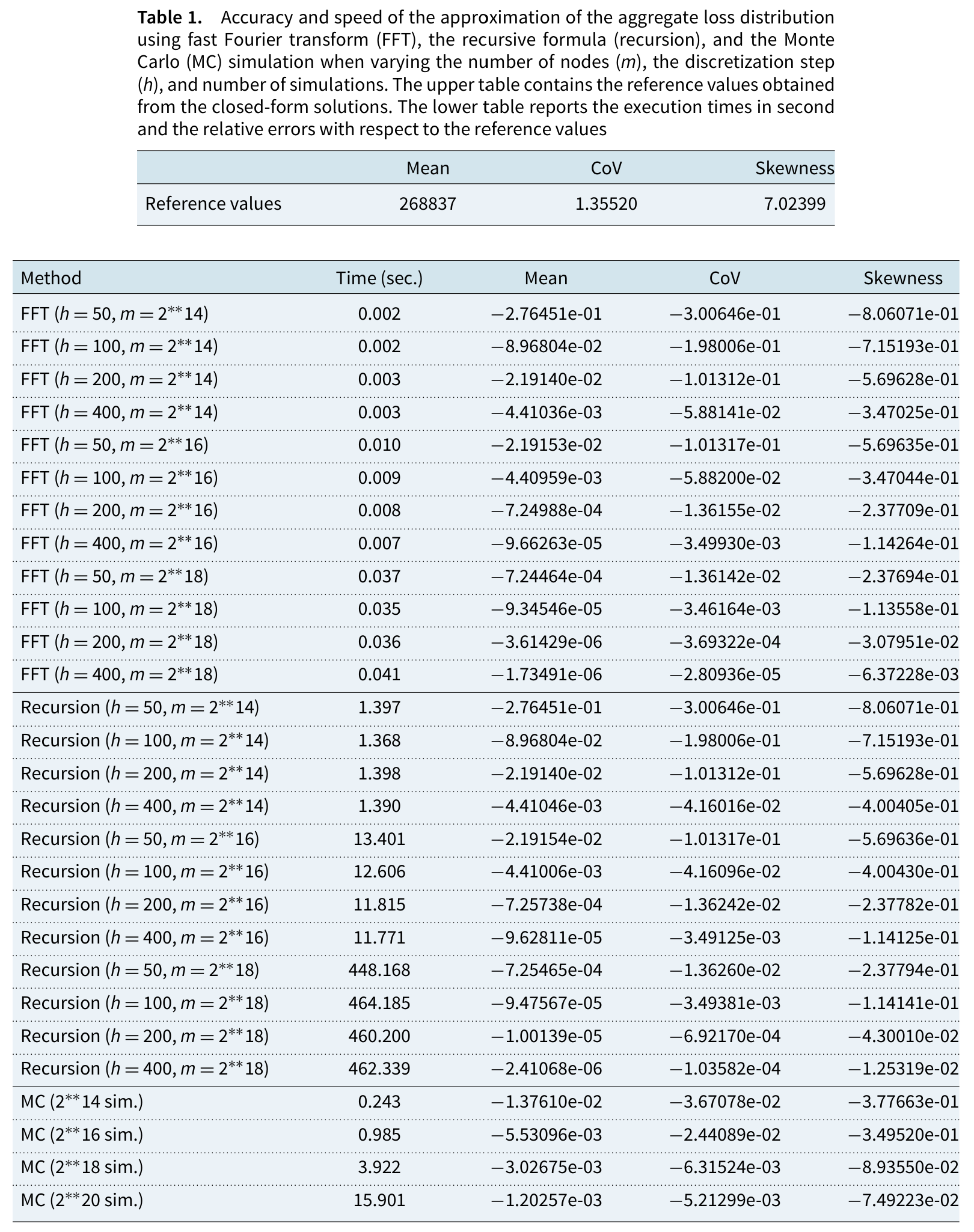
TABLE1 = pd.DataFrame([
    # h, log2 m, FFT mean, CV, skewness errors, recursion mean, CV, skewness errors
    (50, 14, -2.76451e-01, -3.00646e-01, -8.06071e-01, -2.76451e-01, -3.00646e-01, -8.06071e-01),
    (100, 14, -8.96804e-02, -1.98006e-01, -7.15193e-01, -8.96804e-02, -1.98006e-01, -7.15193e-01),
    (200, 14, -2.19140e-02, -1.01312e-01, -5.69628e-01, -2.19140e-02, -1.01312e-01, -5.69628e-01),
    (400, 14, -4.41036e-03, -5.88141e-02, -3.47025e-01, -4.41046e-03, -4.16016e-02, -4.00405e-01),
    (50, 16, -2.19153e-02, -1.01317e-01, -5.69635e-01, -2.19154e-02, -1.01317e-01, -5.69636e-01),
    (100, 16, -4.40959e-03, -5.88200e-02, -3.47044e-01, -4.41006e-03, -4.16096e-02, -4.00430e-01),
    (200, 16, -7.24988e-04, -1.36155e-02, -2.37709e-01, -7.25738e-04, -1.36242e-02, -2.37782e-01),
    (400, 16, -9.66263e-05, -3.49930e-03, -1.14264e-01, -9.62811e-05, -3.49125e-03, -1.14125e-01),
    (50, 18, -7.24464e-04, -1.36142e-02, -2.37694e-01, -7.25465e-04, -1.36260e-02, -2.37794e-01),
    (100, 18, -9.34546e-05, -3.46164e-03, -1.13558e-01, -9.47567e-05, -3.49381e-03, -1.14141e-01),
    (200, 18, -3.61429e-06, -3.69322e-04, -3.07951e-02, -1.00139e-05, -6.92170e-04, -4.30010e-02),
    (400, 18, -1.73491e-06, -2.80936e-05, -6.37228e-03, -2.41068e-06, -1.03582e-04, -1.25319e-02),
], columns=['h', 'log2 m', 'FFT mean', 'FFT CV', 'FFT skewness',
            'recursion mean', 'recursion CV', 'recursion skewness'])
TABLE1['m h'] = TABLE1['h'] * 2 ** TABLE1['log2 m']

GEMACT = json.loads((BOOK_ROOT / 'bench' / 'pittarello2024_timing_gemact.json')
                    .read_text(encoding='utf-8'))
rerun = {(r['h'], r['m_log2']): r['mean_error'] for r in GEMACT['table1_fft']}
TABLE1['GEMAct FFT mean, rerun'] = [rerun[(h, k)] for h, k in zip(TABLE1['h'], TABLE1['log2 m'])]
by_support = (TABLE1.sort_values(['m h', 'h'])
              .set_index(['m h', 'h', 'log2 m'])
              [['FFT mean', 'recursion mean', 'GEMAct FFT mean, rerun']])
GT(by_support, formatters={c: '{x:.5e}' for c in by_support.columns},
   aligners={'log2 m': 'r'})
4 Comments
4.1 Choose the length of the grid before its spacing
Table 1 is a study of truncation presented as a study of discretization. Its errors are fixed by \(mh\), and when \(h\) grows with \(m\) fixed the grid gets longer, more of the tail fits on it, and the error falls; that is the trend the paper reports. On a grid long enough to hold the distribution, Table 6 shows the opposite and expected trend, error falling as \(h^2\). The lesson is to choose the length of the grid first and its spacing second. A default that sizes the grid from the distribution’s moments does that without being asked, which is why the library’s default grid puts every mean here within \(2 \times 10^{-4}\) of its reference. The same distinction runs through Grübel and Hermesmeier (1999), where mass past the end of the grid wraps around, and Embrechts et al. (1993), where the \(O(h^2)\) rate appears once the support is adequate. Here the mass falls off the end instead.
4.2 Table 2, refreshed
The benchmark was a snapshot of
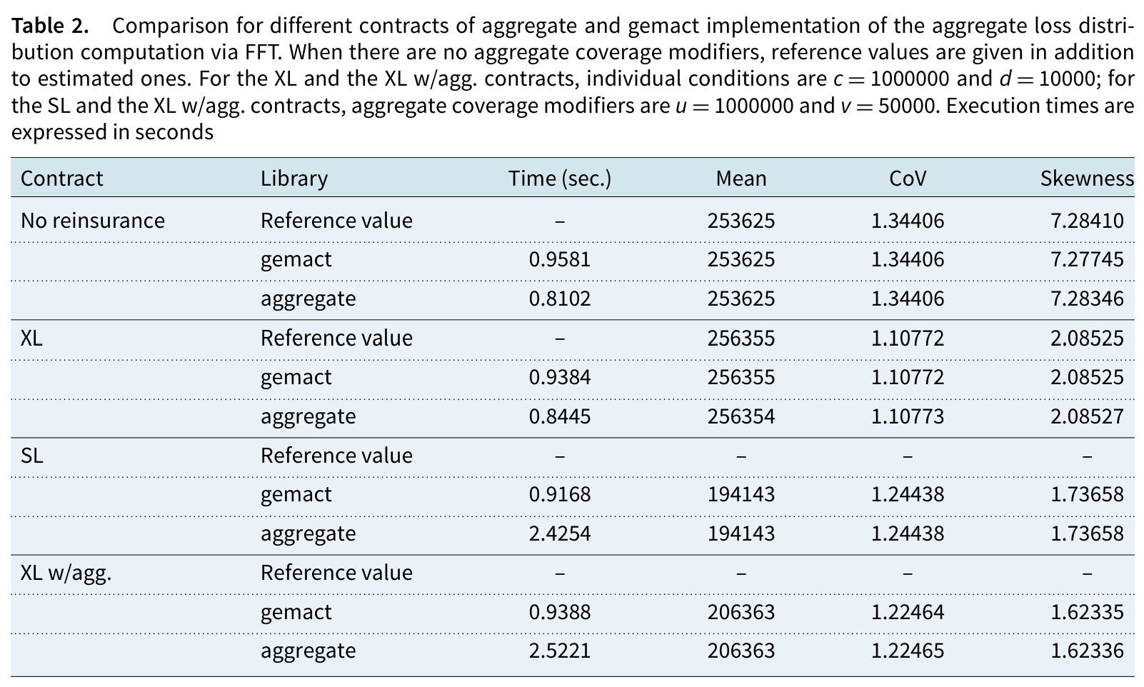
aggregate0.9.3, and its reading, that GEMAct is faster on contracts with aggregate terms at \(2^{22}\) points, still holds on this machine, by a factor of about 1.8 rather than 2.7. The larger difference is the grid. \(2^{22}\) points is sixty-four times the library’s default grid for this portfolio, and on the grid the library chooses for itselfaggregateis about ten times faster than either package at the paper’s size, with means within \(4 \times 10^{-5}\) of the references. The comparison also exposed the skewness defect described above, which the library’s own validation did not catch because it never builds a grid that wide unasked.4.3 Table 3 and copulas
What
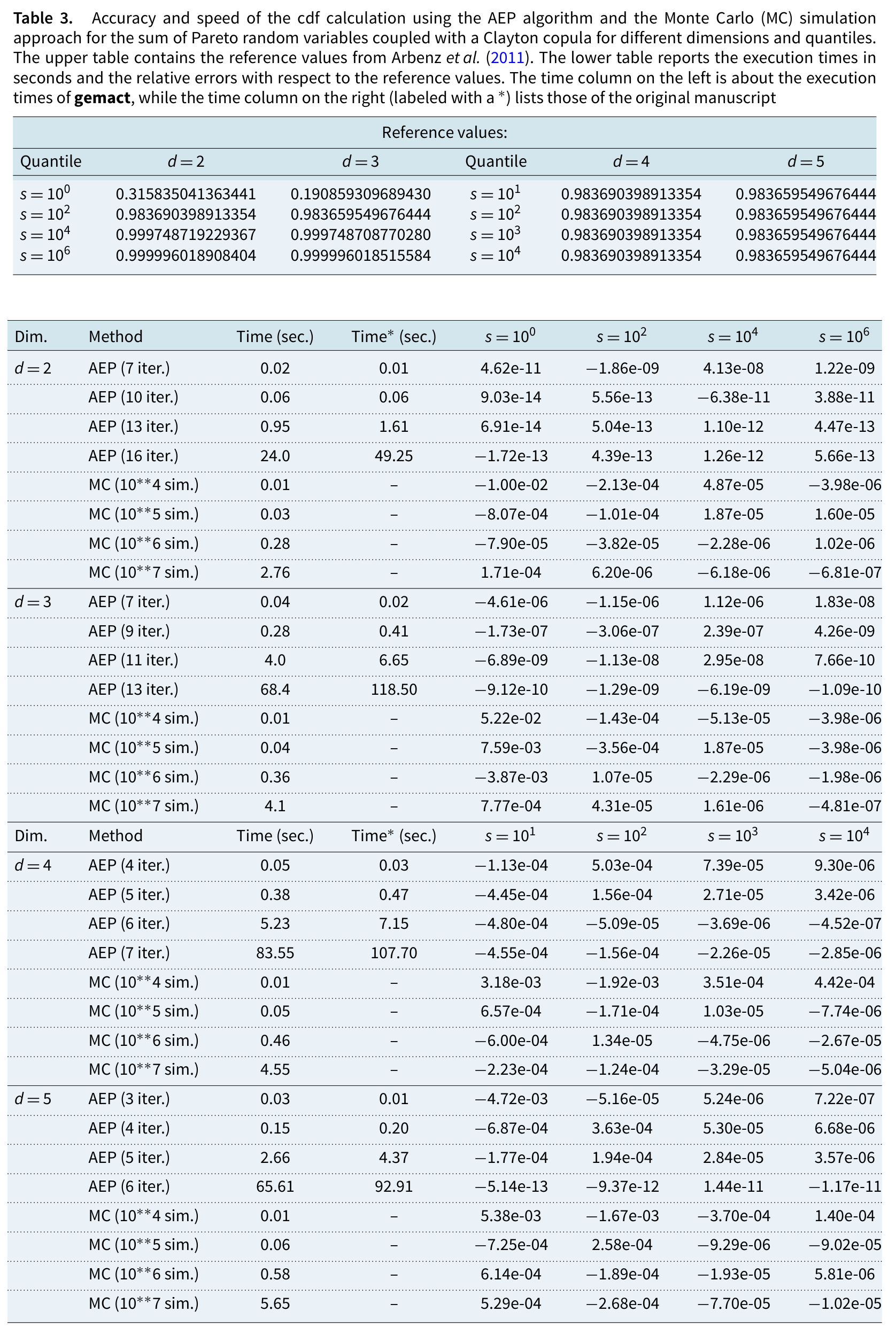
aggregateoffers for dependence is different in kind: a bivariate aggregate with a shared count and a copula on the severities, and Iman-Conover for dependence between lines after each is modeled exactly. Neither is a substitute for AEP on a sum of a few heavy tailed variables. Two smaller points about the reference data are worth recording. Arbenz’s reference values are themselves AEP output at the largest iteration count, sixteen iterations for two dimensions and seven for four, so Table 3’s two dimensional row at sixteen iterations, with errors near \(10^{-13}\), measures agreement between two implementations of the same algorithm rather than accuracy. The four dimensional row at seven iterations, which compares GEMAct with the reference computed at the same setting, shows an error of \(-4.55 \times 10^{-4}\) at \(s = 10\), so there the two implementations disagree.4.4 Out of scope
The reserving module of Section 5 is outside the book’s subject. Figure 1, which compares the four severity discretization methods, is covered by Embrechts and Frei (2009).