Denuit, Ortega-Jiménez and Robert on conditional expectations given the sum
Reproducing Denuit, Ortega-Jiménez and Robert (2025)
Author
Stephen J. Mildenhall
Published
2026-10-22 19:55 commit b5ca906+
1 Context and problem
Given two independent risks \(X\) and \(Y\), write
\[m_X(s) = \mathsf E[X \mid X + Y = s].\]
This is the natural allocation of a pool total back to one of its members, and it is the same object as the previous chapter’s \(\kappa\) and as aggregate’s exeqa_ column. The question Denuit et al. (2025) asks is what \(m_X\) does as \(s\) grows, and the answer turns out to depend on the difference of the two tail indices rather than on either one.
The paper works with densities that are regularly varying: \(f_X\) has index \(\alpha_X\) when it behaves like \(x^{-\alpha_X}\) times a slowly varying factor. Its central results sort into three cases. When \(\alpha_X - \alpha_Y > 1\), \(m_X\) is bounded and must decrease somewhere. When \(\alpha_X - \alpha_Y < 1\), \(m_X\) diverges. The boundary case \(\alpha_X = \alpha_Y + 1\) can go either way, and the limit is \(2\,\mathsf E[X]\), approached from below or from above depending on the slowly varying parts.
The paper is unusually direct about where the question came from. Section 1 records that Mildenhall and Major (2022) “discussed, without proof but providing illustrative examples, the behaviour of \(m_X(\cdot)\) for heavy-tailed losses”, that Section 14.3 of that book states that combining heavy-tailed distributions can produce a humped, non-monotone \(m_X\), and that Example 250 makes a further claim about two random variables. So this chapter is a reproduction of a paper that set out to prove things asserted by example in Pricing Insurance Risk, using the software that generated those examples. That is a closed loop worth checking carefully in both directions.
2 Paper solution and gold standard
The paper prints no tables. Its evidence is a sequence of figures, each with fully specified parameters, plus statements in the text precise enough to check numerically. The three reproduced here are set out in Table 1.
Table 1: The three figures reproduced, their parameters and the claim each makes.
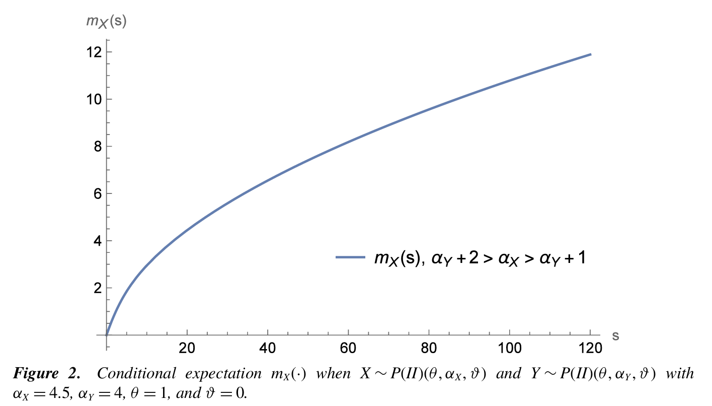
\(m_X\) increases over \((0, 120)\); diverges, since \(\alpha_X - \alpha_Y = 0.5 < 1\)
5
\(P^{(I)}(\theta = 1, \alpha_X = 6)\)
\(P^{(I)}(\theta = 1, \alpha_Y = 5)\)
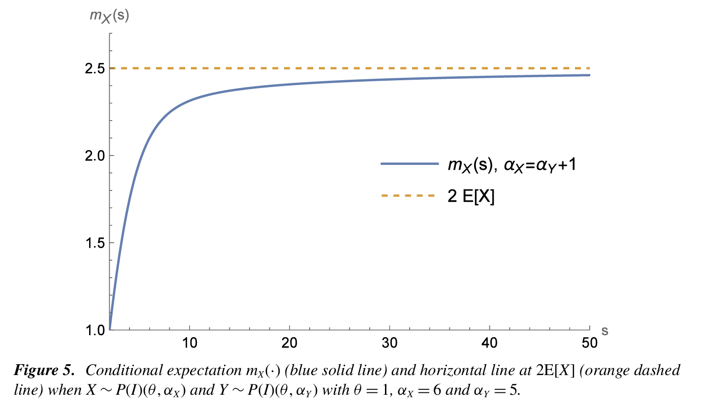
\(m_X\) increases over \((0, 50)\) and tends to \(2\,\mathsf E[X]\)from below
6
\(P^{(I)}(\theta = 1, \alpha_X = 3.5)\)
\(P^{(I)}(\theta = 1, \alpha_Y = 2.5)\)
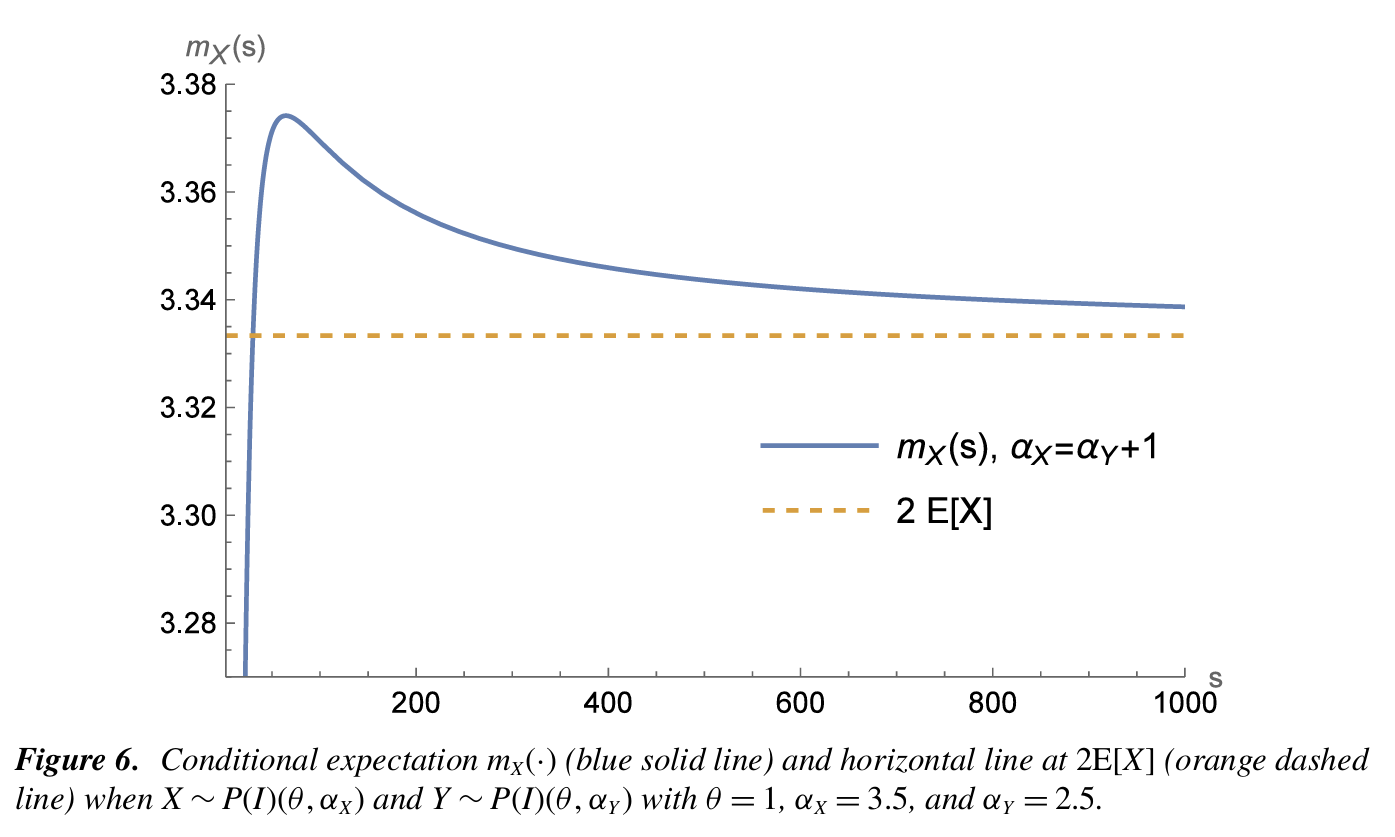
\(m_X\) increases over \((0, 64.46)\), then decreases over \((64.46, 1000)\), tending to \(2\,\mathsf E[X]\)from above
Figure 6, Figure 3, carries the number that makes this reproducible rather than merely plausible: the turning point is at \(64.46 \simeq F^{-1}(0.998)\).
2.1 The one transcription decision, and the number that settles it
\(P^{(I)}\) is the Pareto Type I, supported on \(x > \theta\), and \(P^{(II)}\) is the Lomax, supported on \(x > 0\). Neither identification is in doubt. What is in doubt is the index, because the paper’s \(\alpha\) indexes the density while scipy and DecL take the shape parameter of the survival function, and for a Pareto those differ by one: if \(S_X(x) \sim x^{-a}\) then \(f_X(x) \sim x^{-(a+1)}\). The paper half flags this itself, noting that “Pareto, Log-Gamma, and Dagum distributions are often defined with a parameter \(\beta = \alpha - 1\) instead of the parameter \(\alpha\) which appears in Table 1.”
So the paper’s \(\alpha\) should map to a DecL shape of \(\alpha - 1\). The two readings are not distinguishable from Figures 2 and 5, where both give an increasing curve. Figure 3 distinguishes them, because \(64.46\) is a specific number, and Table 2 is the test.
%xmode minimalimport numpy as npimport pandas as pdimport matplotlib.pyplot as pltfrom aggregate.constants import FIG_W, FIG_Hfrom bookstyle import GT, build, showdef pool(sev_x, sev_y, log2, bs):"""Two independent risks, one claim each, so each aggregate is its severity. The trailer goes on the `port` header line. A trailer written after the last unit binds to that unit, because the portfolio's trailer slot closes before the units are read, and the pool would then be auto-sized. """return build(f'port K hints{{log2={log2}; bs={bs}; normalize=False; padding=1}}\n'f' agg X 1 claim {sev_x} fixed\n'f' agg Y 1 claim {sev_y} fixed\n')def m_x(p, lo, hi):"""m_X on [lo, hi], with the index, as an (index, values) pair.""" k = p.density_df['exeqa_X'] sl = (k.index >= lo) & (k.index <= hi)return k[sl].index.to_numpy(), k[sl].to_numpy()
Exception reporting mode: Minimal
rows = []for label, aX, aY in [('alpha as printed: DecL pareto 3.5 and 2.5', 3.5, 2.5), ('alpha minus one: DecL pareto 2.5 and 1.5', 2.5, 1.5)]: p = pool(f'sev 1 * pareto {aX}', f'sev 1 * pareto {aY}', 20, 0.01) idx, v = m_x(p, 2, 1000) ex = aX / (aX -1) rows.append({'reading': label, 'E[X]': ex, '2 E[X]': 2* ex,'turning point of m_X': idx[v.argmax()],'q(0.998) of S': p.q(0.998),'m_X(1000)': float(p.density_df['exeqa_X'].loc[1000]),'approaches 2E[X] from above':bool(float(p.density_df['exeqa_X'].loc[1000]) >2* ex)})GT(pd.DataFrame(rows).set_index('reading'), float_format=4)
Table 2: The two readings of the paper’s index, each against the three numbers Figure 6 pins down.
reading
E[X]
2 E[X]
turning point of m_X
q(0.998) of S
m_X(1000)
approaches 2E[X] from above
alpha as printed: DecL pareto 3.5 and 2.5
1.4000
2.8000
999.9900
13.8800
2.7987
False
alpha minus one: DecL pareto 2.5 and 1.5
1.6667
3.3333
64.4600
65.3800
3.3387
True
In Table 2, read as printed, there is no turning point inside the range at all: \(m_X\) is still climbing at \(s = 1000\), it approaches its limit from below, and the paper’s \(F^{-1}(0.998)\) comes out at 13.9 rather than 64.46. Read as \(\alpha - 1\), the turning point lands at \(s = 64.46\), the \(99.8\)th percentile of \(S\) is 65.4 against the paper’s “\(\simeq 64.46\)”, and the limit is approached from above. Every one of the paper’s three statements about Figure 6 holds, and none of them holds under the other reading.
That settles the convention for the rest of this page: a printed \(\alpha\) becomes a DecL shape of \(\alpha - 1\).
port Khints{log2=20; bs=0.01; normalize=False; padding=1}agg X1claimsevpareto2.5fixedagg Y1claimsevpareto1.5fixed
rows = []for name, (sx, sy, lg, bs, lo, hi) in FIGS.items(): p = POOLS[name] idx, v = m_x(p, max(lo, p.bs), hi) d = np.diff(v) rows.append({'figure': name, 'E[X]': p.agg_list[0].est_m,'m_X at the left edge': v[0], 'm_X at the right edge': v[-1],'increasing throughout': bool((d >=-1e-9).all()),'turning point': idx[v.argmax()] ifnot (d >=-1e-9).all() else np.nan})GT(pd.DataFrame(rows).set_index('figure'), float_format=4)
Table 3: Each figure’s claim tested: the endpoints of \(m_X\), whether it increases throughout, and any turning point.
figure
E[X]
m_X at the left edge
m_X at the right edge
increasing throughout
turning point
Figure 2
0.4000
0.0010
11.8903
True
—
Figure 5
1.2500
1.0000
2.4600
True
—
Figure 6
1.6667
1.0000
3.3387
False
64.4600
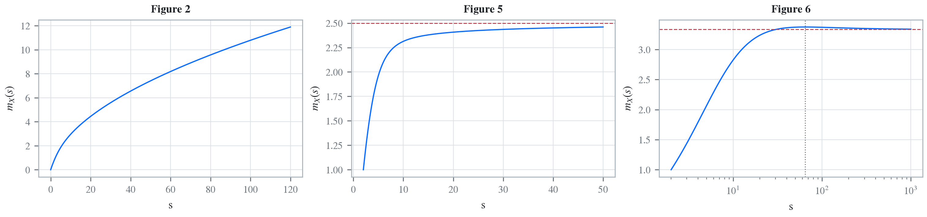
In Table 3, Figure 2 increases over \((0, 120)\) as claimed, and it is the divergent case, so there is nothing for it to converge to. Figure 5 increases over \((2, 50)\) and gets to 2.460 against a limit of \(2\,\mathsf E[X] = 2.5\), approaching from below. Figure 6 turns over at 64.46 and then falls. The published figures are Figure 1, Figure 2 and Figure 3, and Figure 4 is the reproduction.
Figure 1: Denuit, Ortega-Jiménez and Robert (2025), Figure 2.
Figure 2: Denuit, Ortega-Jiménez and Robert (2025), Figure 5.
Figure 3: Denuit, Ortega-Jiménez and Robert (2025), Figure 6.
Figure 4: Reproducing Figures 2, 5 and 6. The dashed line is 2E[X], the limit in the boundary case.
3.1 Figure 6, closely
The paper’s three statements about Figure 3 are all quantitative, so Table 4 checks them one at a time.
p6 = POOLS['Figure 6']k6 = p6.density_df['exeqa_X']idx, v = m_x(p6, 2, 1000)EX6 = p6.agg_list[0].est_mGT(pd.DataFrame([ {'claim': 'turning point', 'paper': '64.46', 'aggregate': f'{idx[v.argmax()]:.2f}'}, {'claim': 'turning point is about the 99.8th percentile of S','paper': '64.46', 'aggregate': f'{p6.q(0.998):.2f}'}, {'claim': 'limit as s grows', 'paper': '2 E[X]', 'aggregate': f'{2* EX6:.5f}'}, {'claim': 'm_X at s = 1000', 'paper': 'above the limit','aggregate': f'{float(k6.loc[1000]):.5f}'}, {'claim': 'increases on (0, 64.46)', 'paper': 'yes','aggregate': str(bool((np.diff(v[:v.argmax() +1]) >=-1e-9).all()))}, {'claim': 'decreases on (64.46, 1000)', 'paper': 'yes','aggregate': str(bool((np.diff(v[v.argmax():]) <=1e-9).all()))},]).set_index('claim'))
Table 4: Every quantitative claim the paper makes about Figure 6, each against the computed value.
claim
paper
aggregate
turning point
64.46
64.46
turning point is about the 99.8th percentile of S
64.46
65.38
limit as s grows
2 E[X]
3.33331
m_X at s = 1000
above the limit
3.33867
increases on (0, 64.46)
yes
True
decreases on (64.46, 1000)
yes
True
In Table 4 the turning point matches to the two decimals printed. That is a strong check: it is a location rather than a level, so it depends on the shape of both densities over the whole range rather than on a normalization, and it would move if either index were wrong.
4 Comments
4.1 The reproduction confirms a book it was written to examine
The paper’s stated motivation is to prove, or qualify, statements made by example in Mildenhall and Major (2022): that combining heavy-tailed distributions can produce a humped, non-monotone conditional expectation given the sum. Figure 3 is that hump, and it reproduces here to the second decimal of its turning point. The examples in Section 14.3 of the book were computed with this library, so the loop closes: an assertion made by numerical example, proved analytically by other authors, and the proof’s own illustration then recovered by the original numerics.
The one thing the reproduction adds is the index convention. Anyone reading the paper’s figures alongside the book’s examples has to know that the paper’s \(\alpha\) is the density index and the book’s is the survival index, and the two differ by one. The 64.46 is what makes that recoverable rather than a matter of taste.
4.2 Reading \(m_X\) in the far tail, and where it stops being real
\(m_X\) is a ratio whose denominator is the density of the sum, so it degrades wherever that density is numerically negligible. aggregate guards this with a noise floor: below EXEQA_NOISE_FLOOR the conditional decomposition is not trusted and the exeqa columns are zeroed rather than allowed to become noise. The visible effect is that \(m_X\) falls off a cliff to zero far past the range where the sum has any probability, and the cliff is an artifact of the guard rather than a property of \(m_X\). Table 5 shows how thin the density gets.
Table 5: \(m_X\) read against the density and survival function of the sum, out to where both are numerically negligible.
s
m_X(s)
p_total(s)
S(s)
10
2.31316
4.643e-07
1.951e-04
50
2.46001
7.457e-11
1.808e-07
100
2.47953
2.157e-12
1.062e-08
200
2.48966
6.490e-14
6.441e-10
400
1.24739
1.990e-15
3.965e-11
800
0.00000
0.000e+00
6.914e-12
The practical rule this suggests is the one the paper itself gives, from a different direction: it suggests checking monotonicity numerically over \((0, b)\) for \(b > \mathsf E[X + Y] + 10^2\sqrt{\mathsf{Var}[X+Y]}\). For a Pareto pair with an index near 2 the variance is large or infinite, so that bound is generous, and the grid has to reach it with resolution left over. Figure 3 needs \(s\) to 1000, which at bs = 0.01 and \(2^{20}\) buckets is comfortable; asking the same grid for \(s\) to \(10^5\) would not be.
4.3 Both readings are worth carrying
The alpha as printed row of Table 2 is not a failure to be hidden. It is the answer to a question a reader will have, and it demonstrates the shape of the mistake: an index off by one on both variables preserves the difference of the indices, so it preserves every one of the paper’s qualitative classifications and changes only the levels and the turning point. A reproduction that checked “does \(m_X\) increase then decrease” would have passed under either reading and learned nothing.
Programs in the aggregate Loss Lab
Each program below opens in the aggregate Loss Lab, which builds it with nothing to install. The names are those in reproductions.agg, where every program is renamed by its paper’s citation key.
Denuit2025.K: a two agent pool where the conditional mean allocation turns over.
Denuit2025.K.v2: a two agent pool where the conditional mean allocation turns over.
Denuit2025.K.v3: a two agent pool where the conditional mean allocation turns over.
Denuit, M. M., Ortega-Jiménez, P., & Robert, C.-Y. (2025). Conditional expectations given the sum of independent random variables with regularly varying densities. ASTIN Bulletin. https://doi.org/10.1017/asb.2025.11
Mildenhall, S. J., & Major, J. A. (2022). Pricing Insurance Risk: Theory and Practice. John Wiley & Sons, Inc. https://doi.org/10.1002/9781119756538
4 Comments
4.1 The reproduction confirms a book it was written to examine
The paper’s stated motivation is to prove, or qualify, statements made by example in Mildenhall and Major (2022): that combining heavy-tailed distributions can produce a humped, non-monotone conditional expectation given the sum. Figure 3 is that hump, and it reproduces here to the second decimal of its turning point. The examples in Section 14.3 of the book were computed with this library, so the loop closes: an assertion made by numerical example, proved analytically by other authors, and the proof’s own illustration then recovered by the original numerics.
The one thing the reproduction adds is the index convention. Anyone reading the paper’s figures alongside the book’s examples has to know that the paper’s \(\alpha\) is the density index and the book’s is the survival index, and the two differ by one. The 64.46 is what makes that recoverable rather than a matter of taste.
4.2 Reading \(m_X\) in the far tail, and where it stops being real
\(m_X\) is a ratio whose denominator is the density of the sum, so it degrades wherever that density is numerically negligible.
aggregateguards this with a noise floor: belowEXEQA_NOISE_FLOORthe conditional decomposition is not trusted and theexeqacolumns are zeroed rather than allowed to become noise. The visible effect is that \(m_X\) falls off a cliff to zero far past the range where the sum has any probability, and the cliff is an artifact of the guard rather than a property of \(m_X\). Table 5 shows how thin the density gets.The practical rule this suggests is the one the paper itself gives, from a different direction: it suggests checking monotonicity numerically over \((0, b)\) for \(b > \mathsf E[X + Y] + 10^2\sqrt{\mathsf{Var}[X+Y]}\). For a Pareto pair with an index near 2 the variance is large or infinite, so that bound is generous, and the grid has to reach it with resolution left over. Figure 3 needs \(s\) to 1000, which at
bs = 0.01and \(2^{20}\) buckets is comfortable; asking the same grid for \(s\) to \(10^5\) would not be.4.3 Both readings are worth carrying
The
alpha as printedrow of Table 2 is not a failure to be hidden. It is the answer to a question a reader will have, and it demonstrates the shape of the mistake: an index off by one on both variables preserves the difference of the indices, so it preserves every one of the paper’s qualitative classifications and changes only the levels and the turning point. A reproduction that checked “does \(m_X\) increase then decrease” would have passed under either reading and learned nothing.