Wilson and Keich (2016) asks a narrow question with a wide answer: given two non-negative vectors, can you compute their convolution by FFT and guarantee the relative accuracy of every entry?
The answer is yes, and the algorithm is aFFT-C. It matters here because aggregate computes compound distributions by exactly the FFT convolution these authors show is unreliable, and because the companion paper Ben Rached et al. (2024) reaches the same conclusion by a different route and recommends abandoning the FFT entirely. This paper does not. It keeps the FFT and fixes it, which is the better outcome for a library that needs \(O(N \log N)\).
The mechanism has three parts:
A computable error bound. For each output index, a bound on the FFT roundoff error that can be evaluated at runtime. This is the part that matters most, because it converts a silent failure into a detected one.
PITS (partitioning into thin slices). Decompose each input pmf into components of reduced dynamic range, so that FFT-C applied to each pair is accurate, then reassemble. Roundoff cannot swamp small values if the small values are never in the same vector as the large ones.
An exponential shift. Precondition by \(p_\theta(k) = p(k)e^{k\theta}/M_p(\theta)\), which commutes with convolution, so it can be peeled off afterward. Its role here is to reduce the number of slices PITS needs, and hence the number of FFT calls.
2 What is reproducible
Table / result
Content
Reproducible
Section 1 toy example
A four-element pmf with exact rational convolution, and the measured relative errors of NC, FFT-C and aFFT-C
Yes, and now exactly: the reference column is library-computed rational arithmetic
Table 1
Number of PITS splits with and without the exponential shift
No, internal to aFFT-C
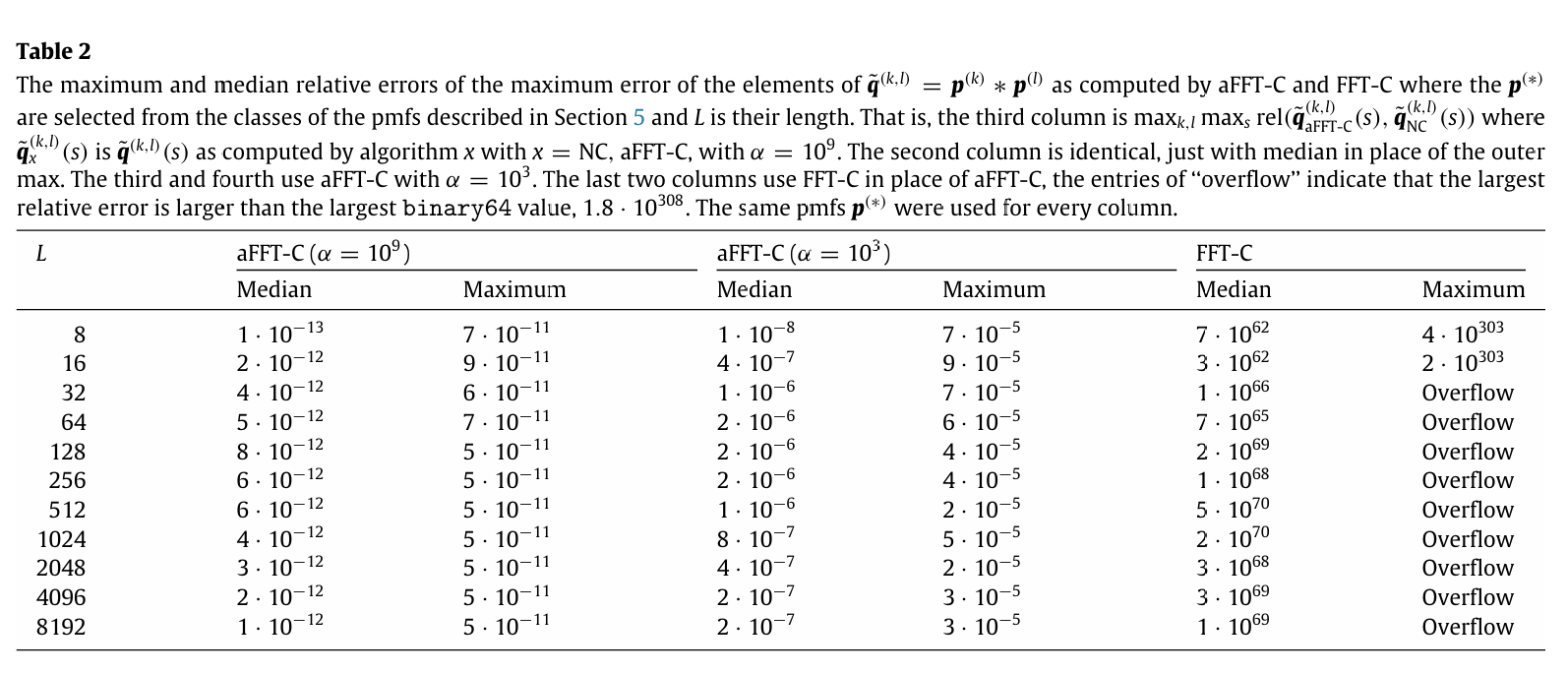
Table 2
Median and maximum relative error of aFFT-C and FFT-C over six declared pmf classes
The FFT-C columns, statistically
Figures 4 and 5
Timing of aFFT-C against naive convolution and FFT-C
No, implementation timing
The aFFT-C columns of Table 2 are not reproducible without implementing aFFT-C. The FFT-C columns are, because FFT-C is what aggregate already does.
3 The Section 1 example
This is the whole paper in seven numbers. Take \(p = (0, a, b, c)\) with \(b = 10^{-5}\), \(c = 10^{-20}\) and \(a = 1 - b - c\). Then
which is exact and needs no numerics at all. The last two entries are \(2 \times 10^{-25}\) and \(10^{-40}\), both far below double precision machine epsilon relative to the leading entry of \(1\).
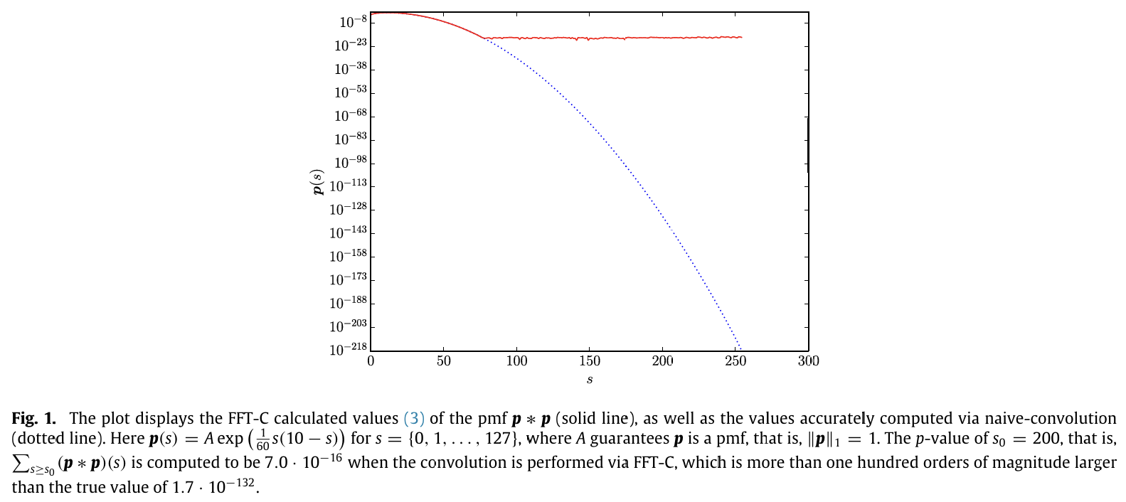
Figure 1 is the paper’s own illustration, and Table 1 recomputes it three ways.
Figure 1: Wilson and Keich (2016), Figure 1, illustrating the Section 1 example.
%xmode minimalimport numpy as npimport pandas as pdfrom functools import partialfrom bookstyle import GT, build# Tail probabilities and relative errors read as powers of ten, not SI prefixes.GT = partial(GT, eng_style='exp')b, c =1e-5, 1e-20a =1- b - cexact = np.array([0.0, 0.0, a * a, 2* a * b, 2* a * c + b * b, 2* b * c, c * c])naive = np.convolve([0, a, b, c], [0, a, b, c]) # NCfftc = np.fft.irfft(np.fft.rfft([0, a, b, c], 8) **2, 8)[:7] # FFT-C# the same convolution through aggregate: a three-point severity, two claimsobj = build(f'agg Toy dfreq [2] dsev [1 2 3] [{a!r}{b!r}{c!r}]', log2=6, bs=1, normalize=False)agg = np.array([obj.agg_density[k] for k inrange(7)])def rel(x):return np.where(exact >0, np.abs(x - exact) / np.where(exact >0, exact, 1.0), 0.0)GT(pd.DataFrame({'k': range(7), 'exact': exact, 'NC': naive, 'FFT-C': fftc,'agg': agg, 'rel NC': rel(naive), 'rel FFT-C': rel(fftc),'rel agg': rel(agg)}))
Exception reporting mode: Minimal
Table 1: The seven entry convolution exactly, by naive convolution, by textbook FFT-C and through the library, with relative errors.
Naive convolution is exact here. The paper reports \(r_{NC,64} = (0, 0, 2\cdot 10^{-16}, 10^{-20}, 2\cdot 10^{-16}, 10^{-16}, 3\cdot 10^{-17})\), and this run gives zero throughout because the individual products happen to be exactly representable. Either way the point stands: NC preserves relative accuracy at every entry, because a sum of non-negative products has no cancellation.
FFT-C destroys the last two entries. Index 5 has a relative error around \(10^{8}\) and index 6 around \(10^{23}\). Both computed values are negative, which is impossible for a convolution of non-negative vectors.
aggregate behaves exactly like textbook FFT-C. Same failure at the same two indices, same orders of magnitude of error. The signs differ, agg returning a positive value at index 5 where FFT-C returns a negative one, because the sign of accumulated rounding is arbitrary and the two routines pad and transform slightly differently. That is the confirmation that agg’s engine is FFT-C and inherits its properties without modification, and also a warning that a negative-value check catches only some of these failures.
Note also index 4, where the true value is \(10^{-10}\): FFT-C is already wrong in the seventh significant figure and agg in the sixth. The degradation is gradual on the way down to the cliff, not sudden.
For contrast the paper reports what aFFT-C achieves on this example:
Every entry to eleven significant figures or better, including the \(10^{-40}\) one, at \(O(N \log N)\) cost.
4 The Section 1 example, exactly
Since this chapter was written the library has grown an exact engine. The DecL kind nttagg computes a bounded discrete compound with no floating point at all: input probabilities are parsed text-exactly as rational numbers, the convolution runs over 32-bit prime fields via the number-theoretic transform, and the answer is reconstructed by the Chinese remainder theorem as exact integer numerators over one common denominator. The float FFT pipeline still runs beside it, driven from the same spec, so one object carries both the textbook computation and the exact answer it should have produced.
That changes the status of this example. The exact column of Table 1 was hand algebra, trustworthy because the convolution has seven entries. It is now library output, and the hand algebra becomes the check on the library rather than the reference for it.
from fractions import Fractionb = Fraction(1, 10**5)c = Fraction(1, 10**20)a =1- b - cwil = build(f'nttagg Wilson dfreq [2] dsev [1 2 3] [{a}{b}{c}]')closed_form = [a * a, 2* a * b, 2* a * c + b * b, 2* b * c, c * c]nonzero = wil.p_exact[wil.p_exact !=0]assertlist(nonzero) == closed_form, 'library p_exact differs from the closed form'print('p_exact == [a^2, 2ab, 2ac + b^2, 2bc, c^2] as exact Fractions: True')GT(wil.density_df.query('p_exact_float > 0')[['p_total', 'p_exact_float', 'p_exact_log10']])
Table 2: The Section 1 example computed exactly by the library. The exact column matches the closed form identically, as Fractions, and p_exact_log10 resolves the entries that are invisible to a double.
loss
p_total
p_exact_float
p_exact_log10
2
999.980e-03
999.980e-03
-8.686e-06
3
20.000e-06
20.000e-06
-4.699e+00
4
100.000e-12
100.000e-12
-10.000e+00
5
0.000e+00
200.000e-27
-24.699e+00
6
0.000e+00
100.000e-42
-40.000e+00
Two readings of Table 2. First, the assert passed: the five nonzero probabilities the engine reconstructs equal \((a^2,\ 2ab,\ 2ac + b^2,\ 2bc,\ c^2)\) as exact rational numbers, not to any tolerance. Second, p_total, the float pipeline’s answer inside the same object, reads exactly zero at losses 5 and 6, where the truth is \(2\times 10^{-25}\) and \(10^{-40}\). The float pipeline does not merely get these entries wrong; after cleanup it reports them as structurally absent.
The paper’s central contribution is a runtime certificate: a computable bound that tells the caller which entries of an FFT convolution are trustworthy. On this envelope, nonnegative integer outcomes with bounded support and rational probabilities, the library now does something categorically stronger. It does not bound the error of the float pipeline; it computes it, per bucket, exactly before the final rounding. Table 3 is the paper’s Figure 1 regenerated from inside the library.
GT(wil.accuracy_df.loc[2:6])
Table 3: The per-bucket error of the float FFT pipeline against the exact answer, computed exactly. p_fft is the raw signed FFT output before cleanup, and the relative errors at losses 5 and 6 are the catastrophe the paper exhibits.
loss
p_exact_float
p_fft
err
abs_err
rel_err
2
999.980e-03
999.980e-03
9.93e-17
9.93e-17
9.93e-17
3
20.000e-06
20.000e-06
-4.30e-17
4.30e-17
-2.15e-12
4
100.000e-12
100.000e-12
-2.04e-17
2.04e-17
-2.04e-07
5
200.000e-27
18.316e-18
1.83e-17
1.83e-17
9.16e+07
6
100.000e-42
27.756e-18
2.78e-17
2.78e-17
2.78e+23
The relative errors at losses 5 and 6 in Table 3 are the failures of Table 1, now library-reported rather than hand-measured, and p_fft preserves the raw signed noise that p_total clips, so the arbitrary sign discussed under Table 1 is visible too.
4.1 Adjudicating the naive convolution claim
The discussion under Table 1 noted a small discrepancy with the paper: the paper reports nonzero relative errors for naive convolution, around \(10^{-16}\), while our run measured zero throughout. With an exact yardstick the discrepancy resolves, and both observations turn out to be right.
af, bf, cf =float(a), float(b), float(c)naive_f = np.convolve([0, af, bf, cf], [0, af, bf, cf])float_form = [af * af, 2* af * bf, 2* af * cf + bf * bf, 2* bf * cf, cf * cf]rows = []for k inrange(2, 7): e = closed_form[k -2] rows.append({'k': k, 'NC': naive_f[k],'rel err vs float closed form':float((Fraction(naive_f[k]) - Fraction(float_form[k -2])) / e),'rel err vs exact':float((Fraction(naive_f[k]) - e) / e)})GT(pd.DataFrame(rows))
Table 4: Naive convolution against two yardsticks. Against the float evaluation of the closed form it is bit-identical; against the exact rational answer it carries the input representation error, which is what the paper’s r_NC reports.
k
NC
rel err vs float closed form
rel err vs exact
2
999.980e-03
0
9.93e-17
3
20.000e-06
0
5.99e-17
4
100.000e-12
0
2.21e-16
5
200.000e-27
0
3.85e-17
6
100.000e-42
0
-7.07e-17
In Table 4 the middle column is identically zero: the doubles naive convolution returns are bit-for-bit the float evaluation of the closed form, so the arithmetic commits no error at all, which is the no-cancellation property the paper proves. The right column sits at \(10^{-16}\) to \(10^{-17}\), and every bit of it is the cost of writing \(a\), \(b\), \(c\) as doubles in the first place, before any arithmetic runs. The paper’s \(r_{NC,64} = (0, 0, 2\cdot 10^{-16}, 10^{-20}, 2\cdot 10^{-16}, 10^{-16}, 3\cdot 10^{-17})\) is the same quantity measured on its authors’ machine. Our earlier “zero throughout” was an artifact of a yardstick that was itself computed in doubles and therefore shared the inputs’ rounding.
5 Table 2: the FFT-C columns
Table 2, Figure 2, measures relative error over six pmf classes, which the paper defines precisely. With \(a, b, c \sim U(0,1)\) fixed per pmf, \(u_i \sim U(0,1)\) per entry, and \(A\) normalizing:
constant, \(p(i) \equiv A\)
random, \(p(i) = A\exp(-40u_i)\)
quadratic, \(p(i) = A\exp(-30(a+1)x_i^2 + 20(2b-1)x_i + 20(2c-1))\), \(x\) even on \([0,1]\)
sinusoid, \(p(i) = A\exp(10(3a+1)\sin(x_i + b/10) + 10(5c-4)x_i)\), \(x\) even on \([0, 3\pi]\)
multi-scaled I, a random fifth are \(A\exp(-30u_i)\), the rest \(A\exp(-100(u_i+1))\)
multi-scaled II, a random third are \(A\exp(-15(2a+1)u_i)\), the rest \(A\exp(-50((2a+1)u_i + 2b + 1))\)
Figure 2: Wilson and Keich (2016), Table 2.
from scipy.special import logsumexprng = np.random.default_rng(20260806)N_DRAW =12# the paper uses 100 per classdef make(cls, L, rng): a_, b_, c_ = rng.uniform(size=3) u = rng.uniform(size=L)if cls ==1: lv = np.zeros(L)elif cls ==2: lv =-40* uelif cls ==3: x = np.linspace(0, 1, L) lv =-30* (a_ +1) * x **2+20* (2* b_ -1) * x +20* (2* c_ -1)elif cls ==4: x = np.linspace(0, 3* np.pi, L) lv =10* (3* a_ +1) * np.sin(x + b_ /10) +10* (5* c_ -4) * xelif cls ==5: idx = rng.permutation(L) lv =-100* (u +1) lv[idx[:L //5]] =-30* u[idx[:L //5]]else: idx = rng.permutation(L) lv =-50* ((2* a_ +1) * u +2* b_ +1) lv[idx[:L //3]] =-15* (2* a_ +1) * u[idx[:L //3]]return np.exp(lv - logsumexp(lv))published = {8: ('7e62', '4e303'), 128: ('2e69', 'Overflow'),1024: ('2e70', 'Overflow'), 8192: ('1e69', 'Overflow')}rows = []for L in [8, 128, 1024, 8192]: worst, per_pair =0.0, []for cls inrange(1, 7): ps = [make(cls, L, rng) for _ inrange(N_DRAW)]for i inrange(N_DRAW):for j inrange(i, N_DRAW): ex = np.convolve(ps[i], ps[j]) nq =1<<int(np.ceil(np.log2(2* L -1))) ap = np.fft.irfft(np.fft.rfft(ps[i], nq)* np.fft.rfft(ps[j], nq), nq)[:2* L -1] ok = ex >0 r = np.abs(ap[ok] - ex[ok]) / ex[ok] per_pair.append(r.max()) worst =max(worst, r.max()) pm, px = published[L] rows.append({'L': L, 'FFT-C median (here)': np.median(per_pair),'FFT-C max (here)': worst,'paper median': pm, 'paper max': px})GT(pd.DataFrame(rows))
Table 5: FFT-C relative error over the six pmf classes at four lengths, beside the median and maximum Table 2 reports.
L
FFT-C median (here)
FFT-C max (here)
paper median
paper max
8
23.123e+30
361.344e+288
7e62
4e303
128
5.998e+33
7.114e+225
2e69
Overflow
1,024
130.059e+27
1.438e+177
2e70
Overflow
8,192
30.762e+42
1.461e+276
1e69
Overflow
Qualitatively Table 5 is an exact reproduction: FFT-C’s relative error on these classes is astronomically large at every length, and the maxima run into the hundreds of orders of magnitude. Quantitatively it is not a close match. The medians here are around \(10^{29}\) to \(10^{43}\) against the paper’s \(10^{62}\) to \(10^{70}\). With 12 draws per class rather than 100, a different generator, and a statistic that spans three hundred orders of magnitude, that gap is unsurprising and I would not read anything into it. This block establishes the regime, not the digits.
6 Discussion
The result that matters for aggregate is not the size of the error but its detectability. In Table 1 the two wrong entries came back negative, which is a free diagnostic. In general they do not: FFT-C can return a plausible positive number that is wrong by a hundred orders of magnitude, with nothing in the output to indicate it.
That is the gap aFFT-C closes. Its contribution is less the slicing than the runtime bound, which lets the algorithm report which indices are trustworthy. A convolution routine that returns values and a certificate is categorically more useful than one that returns values alone, and it is the piece aggregate currently lacks. The refinement heuristic used on the Ben Rached et al. (2024) page, build twice and compare, is a poor substitute: it costs a second build and it only detects instability, not error.
Two caveats on transferring this wholesale. First, the paper’s setting is pairwise convolution of two arbitrary lattice pmfs, whereas aggregate iterates one severity against itself under a frequency distribution, which is the setting of the companion paper Wilson and Keich (2017). Second, the dynamic ranges here are extreme by construction. Classes 5 and 6 mix components differing by \(e^{-100}\) against \(e^{-30}\), which is far beyond a severity curve. The failure is real, but the test problems are adversarial, and an actuarial severity is closer to the benign end.
Where this bites in practice is not a pathological pmf but an ordinary one evaluated far into a tail, which is exactly what Wilson and Keich (2017) addresses.
Since this chapter was written the gap it identifies has closed, on this paper’s own terrain. The nttagg kind computes a bounded discrete compound exactly, in rational arithmetic over prime fields, and reports the float pipeline’s error per bucket, exactly, in accuracy_df. On the lattice, the library now returns values and something stronger than a certificate: the error itself. What aFFT-C’s bound still offers that the exact engine does not is generality, since the exact route needs rational inputs, integer outcomes and bounded support, while the bound asks nothing of the pmf. For the continuous severities and unbounded frequencies that make up ordinary actuarial work, the runtime bound remains the relevant idea and remains unimplemented.
Programs in the aggregate Loss Lab
Each program below opens in the aggregate Loss Lab, which builds it with nothing to install. The names are those in reproductions.agg, where every program is renamed by its paper’s citation key.
Wilson2016a.Toy: the adversarial severity that breaks naive FFT convolution.
Wilson2016a.Wilson: the adversarial severity that breaks naive FFT convolution.
Ben Rached, N., Hoel, H., & Meo, J. V. (2024). A fast and accurate numerical method for the left tail of sums of independent random variables. Statistics and Computing. https://doi.org/10.1007/s11222-024-10514-5
Wilson, H., & Keich, U. (2016). Accurate pairwise convolutions of non-negative vectors via FFT. Computational Statistics and Data Analysis, 101, 300–315. https://doi.org/10.1016/j.csda.2016.03.010
Wilson, H., & Keich, U. (2017). Accurate small tail probabilities of sums of iid lattice-valued random variables via FFT. Journal of Computational and Graphical Statistics, 26(1), 223–229.