Bruno et al. on thresholded direct convolution

Reproducing Bruno, Camerini, Manna and Tomassetti (2006)

1 Context and problem

Bruno et al. (2006) proposes a direct method for the aggregate claims distribution, competing with Panjer recursion, De Pril transforms and the FFT. The idea is thresholded direct convolution: at each convolution order, keep only the outcomes whose probability exceeds a cutoff chosen so that the retained mass and the first three moments are correct to a prescribed tolerance, here \(10^{-6}\), and discard the rest.

The claimed advantages are that no assumption is needed on the counting distribution, that severities need not be identically distributed, and that the method avoids the underflow that kills Panjer recursion at large \(\lambda\) and the overflow and bit-reversal overhead of the FFT. Tables 3 to 5 count multiplications, Table 4 reports timings, and the authors conclude their method is “more flexible, easier and cheaper than the (exact and approximated) methods using recursion and FFT”, with the advantage growing as the number of convolutions rises.

This is a method paper of the most useful kind for a reproduction: it gives the full input specification and tabulates the output distribution to six decimal places.

2 Paper solution and gold standard

Severity is a 14-point discrete law on the integers 14 to 60, Figure 1, the same for every claim. The three counting distributions are set out in Table 1.

Table 1: The three published tables, their counting distributions and what each tabulates.

Table	Counting distribution	Content
6	Poisson, \(\lambda = 504.814259\)	probability and CDF at 28 quantiles
7	Poisson, \(\lambda = 91{,}000\)	CDF at 28 quantiles, 92,832 convolutions
8	Poisson mixed by a generalized Pareto	CDF at 17 quantiles

The quantiles are quoted as \(\mu + k\sigma\) for stated \(\mu\) and \(\sigma\) and then truncated to integers, so the comparison is unambiguous: evaluate at the integers printed. Table 2 checks the transcribed severity first.

Figure 1: Bruno et al (2006), Table 1.

%xmode minimal
import numpy as np
import pandas as pd
from scipy.integrate import quad
from scipy.special import gammaln
from bookstyle import GT, build

XS = [14, 15, 16, 17, 18, 19, 20, 24, 26, 28, 30, 31, 55, 60]
PS = [.0103301, .0307990, .0293511, .0103301, .0730414, .0111568, .0264554,
      .1002133, .0815418, .0252146, .0212857, .0254214, .0991756, .4556837]
DSEV = ('dsev [' + ' '.join(map(str, XS)) + '] ['
        + ' '.join(f'{q:.7f}' for q in PS) + ']')
x, p = np.array(XS, float), np.array(PS)
m1, m2 = (x * p).sum(), (x ** 2 * p).sum()
GT(pd.DataFrame([{'sum of probabilities': p.sum(), 'severity mean': m1,
                  'E[U^2]': m2, 'severity sd': np.sqrt(m2 - m1 ** 2)}]),
   formatters={'sum of probabilities': 10, 'severity mean': 6, 'E[U^2]': 4,
               'severity sd': 6})

Exception reporting mode: Minimal

Table 2: The transcribed 14 point severity, its total mass and its first two moments.

sum of probabilities	severity mean	E[U^2]	severity sd
1.0000000000	42.761197	2,174.3969	18.597766

3 Table 6: Poisson, \(\lambda = 504.814259\)

The severity is integer valued, so the aggregate lives on the integer lattice and bs = 1 is exact. The support runs to \(658 \times 60 = 39{,}480\), comfortably inside \(2^{17}\). The target is Figure 2.

Figure 2: Bruno et al (2006), Table 6.

LAM6 = 504.814259
a6 = build(f'agg B {LAM6} claims {DSEV} poisson', log2=17, bs=1,
           padding=1, normalize=False)
GT(pd.DataFrame([
    {'quantity': 'mean', 'aggregate': a6.est_m, 'lambda E[U]': LAM6 * m1,
     'paper': 21586.462129},
    {'quantity': 'standard deviation', 'aggregate': a6.est_sd,
     'lambda E[U]': np.sqrt(LAM6 * m2), 'paper': 1047.695834},
    {'quantity': 'total mass', 'aggregate': a6.agg_density.sum(),
     'lambda E[U]': 1.0, 'paper': 1.0},
]).set_index('quantity'), float_format=6)

Table 3: The Table 6 aggregate’s mean, standard deviation and total mass, against the compound Poisson formulas and the printed values.

quantity	aggregate	lambda E[U]	paper
mean	21,586.462129	21,586.462129	21,586.462129
standard deviation	1,047.695834	1,047.695834	1,047.695834
total mass	1.000000	1.000000	1.000000

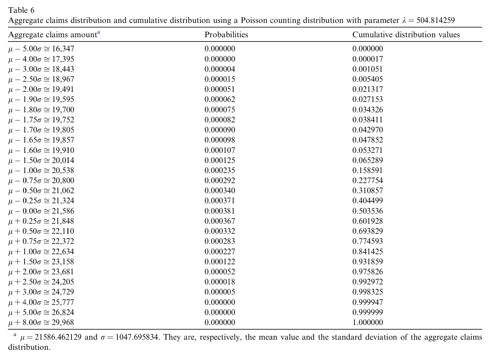
T6 = [(16347, .000000, .000000), (17395, .000000, .000017),
      (18443, .000004, .001051), (18967, .000015, .005405),
      (19491, .000051, .021317), (19595, .000062, .027153),
      (19700, .000075, .034326), (19752, .000082, .038411),
      (19805, .000090, .042970), (19857, .000098, .047852),
      (19910, .000107, .053271), (20014, .000125, .065289),
      (20538, .000235, .158591), (20800, .000292, .227754),
      (21062, .000340, .310857), (21324, .000371, .404499),
      (21586, .000381, .503536), (21848, .000367, .601928),
      (22110, .000332, .693829), (22372, .000283, .774593),
      (22634, .000227, .841425), (23158, .000122, .931859),
      (23681, .000052, .975826), (24205, .000018, .992972),
      (24729, .000005, .998325), (25777, .000000, .999947),
      (26824, .000000, .999999), (29968, .000000, 1.000000)]
d6 = a6.density_df
t6 = pd.DataFrame([{'x': xx, 'agg probability': d6.loc[xx, 'p_total'],
                    'Table 6 probability': pp, 'agg CDF': d6.loc[xx, 'F'],
                    'Table 6 CDF': cc} for xx, pp, cc in T6])
t6['CDF diff'] = (t6['agg CDF'] - t6['Table 6 CDF']).abs()
GT(t6.set_index('x'),
   formatters={'agg probability': 6, 'Table 6 probability': 6, 'agg CDF': 6,
               'Table 6 CDF': 6, 'CDF diff': '{x:.2e}'})

Table 4: All 28 rows of Table 6, probability and CDF, against the rebuilt values.

x	agg probability	Table 6 probability	agg CDF	Table 6 CDF	CDF diff
16,347	0.000000	0.000000	0.000000	0.000000	8.07e-08
17,395	0.000000	0.000000	0.000017	0.000017	4.68e-08
18,443	0.000004	0.000004	0.001051	0.001051	2.56e-07
18,967	0.000015	0.000015	0.005405	0.005405	1.86e-07
19,491	0.000051	0.000051	0.021317	0.021317	1.31e-07
19,595	0.000062	0.000062	0.027153	0.027153	1.15e-07
19,700	0.000075	0.000075	0.034326	0.034326	4.11e-08
19,752	0.000082	0.000082	0.038411	0.038411	1.71e-07
19,805	0.000090	0.000090	0.042970	0.042970	4.49e-07
19,857	0.000098	0.000098	0.047852	0.047852	3.09e-07
19,910	0.000107	0.000107	0.053271	0.053271	2.19e-07
20,014	0.000125	0.000125	0.065289	0.065289	2.51e-07
20,538	0.000235	0.000235	0.158591	0.158591	4.03e-07
20,800	0.000292	0.000292	0.227754	0.227754	3.37e-07
21,062	0.000340	0.000340	0.310857	0.310857	2.39e-07
21,324	0.000371	0.000371	0.404499	0.404499	2.45e-08
21,586	0.000381	0.000381	0.503536	0.503536	2.36e-07
21,848	0.000367	0.000367	0.601928	0.601928	3.08e-07
22,110	0.000332	0.000332	0.693829	0.693829	3.62e-07
22,372	0.000283	0.000283	0.774593	0.774593	5.32e-08
22,634	0.000227	0.000227	0.841425	0.841425	2.46e-07
23,158	0.000122	0.000122	0.931859	0.931859	4.14e-07
23,681	0.000052	0.000052	0.975826	0.975826	1.41e-07
24,205	0.000018	0.000018	0.992972	0.992972	9.39e-08
24,729	0.000005	0.000005	0.998325	0.998325	3.66e-07
25,777	0.000000	0.000000	0.999947	0.999947	3.70e-07
26,824	0.000000	0.000000	0.999999	0.999999	2.37e-07
29,968	0.000000	0.000000	1.000000	1.000000	2.00e-15

GT(pd.DataFrame([{'rows compared': len(t6),
                  'largest CDF difference': float(t6['CDF diff'].max()),
                  'largest probability difference':
                      float((t6['agg probability']
                             - t6['Table 6 probability']).abs().max())}]),
   formatters={'largest CDF difference': '{x:.2e}',
               'largest probability difference': '{x:.2e}'})

Table 5: Worst difference over Table 6, in both the probability and the CDF column.

rows compared	largest CDF difference	largest probability difference
28	4.49e-07	4.93e-07

In Table 4 and Table 5 both columns match to \(5\times10^{-7}\), which is exact at the six decimals printed. In Table 3 the aggregate mean agrees with \(\lambda \mathsf E[U]\) to twelve digits.

4 Table 8: Poisson mixed by a generalized Pareto

The counting law is \(N \mid \Theta \sim \mathrm{Poisson}(\Theta)\) with \(\Theta\) generalized Pareto, \(a = 3.4959\), \(b = 30.1234\), \(c = 1.99321\), in the Klugman parameterization

\[u(\lambda) = \frac{a^{b}\,\Gamma(b+c)}{\Gamma(b)\Gamma(c)} \cdot \frac{\lambda^{c-1}}{(a+\lambda)^{b+c}}.\]

This mixing family is not one of the built-in mixed frequencies, which cover gamma, inverse Gaussian, Sichel, Delaporte and beta. It does not need to be: the paper’s method and aggregate agree that what a compound distribution needs from the frequency is a probability vector, so compute \(p(n) = \mathsf E[e^{-\Theta}\Theta^n/n!]\) by quadrature and hand it over as a dfreq. The target is Figure 3.

The mixing moments are \(\mathsf E[\Theta] = ac/(b-1)\) and \(\mathsf E[\Theta^2] = a^2 c(c+1)/((b-1)(b-2))\), which give the independent check on the parameterization in Table 6, before any of it is used.

A, B, C = 3.4959, 30.1234, 1.99321
ETH = A * C / (B - 1)
ETH2 = A ** 2 * C * (C + 1) / ((B - 1) * (B - 2))
GT(pd.DataFrame([
    {'quantity': 'E[Theta] = E[N]', 'recomputed': ETH, 'paper': np.nan},
    {'quantity': 'aggregate mean', 'recomputed': ETH * m1, 'paper': 10.2310},
    {'quantity': 'aggregate standard deviation',
     'recomputed': np.sqrt(ETH * m2 + (ETH2 - ETH ** 2) * m1 ** 2),
     'paper': 24.0489},
]).set_index('quantity'), float_format=6)

Table 6: The mixing distribution’s moments, and the aggregate mean and standard deviation they imply, against the paper’s.

quantity	recomputed	paper
E[Theta] = E[N]	0.239260	—
aggregate mean	10.231041	10.231000
aggregate standard deviation	24.048924	24.048900

Figure 3: Bruno et al (2006), Table 8.

lc = np.log(A) * B + gammaln(B + C) - gammaln(B) - gammaln(C)
mix_pdf = lambda lam: np.exp(lc + (C - 1) * np.log(lam)
                             - (B + C) * np.log(A + lam))
pn = np.array([quad(lambda t: np.exp(-t + n * np.log(t) - gammaln(n + 1))
                    * mix_pdf(t), 0, np.inf, limit=400)[0]
               for n in range(401)])
keep = pn > 1e-14
ns, qs = np.arange(401)[keep], pn[keep]
FREQ = ('dfreq [' + ' '.join(map(str, ns)) + '] ['
        + ' '.join(f'{q:.14e}' for q in qs) + ']')
a8 = build(f'agg B8 {FREQ} {DSEV}', log2=16, bs=1, padding=1, normalize=False)

T8 = [(0, .798708), (4, .798708), (10, .798708), (16, .810615), (22, .831052),
      (28, .866018), (34, .874409), (46, .877189), (58, .896084),
      (70, .973562), (82, .980304), (106, .987965), (130, .997091),
      (202, .999813), (250, .999972), (491, 1.000000), (1212, 1.000000)]
t8 = pd.DataFrame([{'x': xx, 'agg CDF': a8.density_df.loc[xx, 'F'],
                    'Table 8 CDF': cc} for xx, cc in T8])
t8['diff'] = (t8['agg CDF'] - t8['Table 8 CDF']).abs()
GT(t8.set_index('x'),
   formatters={'agg CDF': 6, 'Table 8 CDF': 6, 'diff': '{x:.2e}'})

Table 7: All 17 rows of Table 8, the CDF under the generalized Pareto mixed Poisson, against the rebuilt values.

x	agg CDF	Table 8 CDF	diff
0	0.798708	0.798708	4.00e-07
4	0.798708	0.798708	4.00e-07
10	0.798708	0.798708	4.00e-07
16	0.810615	0.810615	4.93e-07
22	0.831052	0.831052	8.92e-08
28	0.866018	0.866018	8.98e-08
34	0.874409	0.874409	4.31e-07
46	0.877189	0.877189	3.67e-07
58	0.896084	0.896084	2.68e-07
70	0.973562	0.973562	6.24e-08
82	0.980304	0.980304	1.06e-07
106	0.987965	0.987965	2.34e-07
130	0.997091	0.997091	2.67e-07
202	0.999813	0.999813	4.88e-08
250	0.999972	0.999972	3.65e-07
491	1.000000	1.000000	2.29e-09
1,212	1.000000	1.000000	2.34e-12

GT(pd.DataFrame([{'counts retained above 1e-14': int(ns[-1]),
                  'sum of p(n)': float(pn.sum()),
                  'p(0)': float(pn[0]), 'Table 8 CDF at 0': 0.798708,
                  'agg mean': a8.est_m, 'agg sd': a8.est_sd,
                  'largest CDF difference': float(t8['diff'].max())}]),
   formatters={'sum of p(n)': 12, 'p(0)': 6, 'Table 8 CDF at 0': 6,
               'agg mean': 6, 'agg sd': 6,
               'largest CDF difference': '{x:.2e}'})

Table 8: The truncated frequency vector, the resulting moments, and the worst error over Table 8.

counts retained above 1e-14	sum of p(n)	p(0)	Table 8 CDF at 0	agg mean	agg sd	largest CDF difference
17	0.999999999998	0.798708	0.798708	10.231042	24.049132	4.93e-07

Table 7 and Table 8 have all seventeen values exact at six decimals, including \(p(0) = 0.798708\), which is the probability of no claim and so the CDF’s value everywhere below 14.

5 Table 7: \(\lambda = 91{,}000\), the case the competitors could not do

This is the paper’s showcase. At \(\lambda = 91{,}000\) the aggregate mean is 3.89 million, the method needs 92,832 convolutions, and Table 4 records that Panjer recursion and De Pril both underflow at \(\lambda\) as low as 1004.8. The authors report 1,950 seconds for their own method here. Their FFT comparison stops at \(\lambda = 5004.8\), where it took 3,850 seconds.

The support runs to \(92{,}832 \times 60 = 5.57\) million, so a grid of \(2^{23}\) at bs = 1 holds it whole and no padding is needed: with the support strictly inside the grid there is nowhere for aliasing to come from. The target is Figure 4.

Figure 4: Bruno et al (2006), Table 7.

import time
t0 = time.time()
a7 = build(f'agg B7 91000 claims {DSEV} poisson', log2=23, bs=1,
           padding=0, normalize=False)
elapsed = time.time() - t0
GT(pd.DataFrame([{'seconds': elapsed, 'grid points': 2 ** 23,
                  'x_max': a7.xs[-1], 'mean': a7.est_m, 'sd': a7.est_sd,
                  'paper mean': 3891268.954300, 'paper sd': 14066.631372,
                  'total mass': a7.agg_density.sum()}]),
   formatters={'seconds': 2, 'grid points': '{x:,.0f}', 'x_max': '{x:,.0f}',
               'mean': '{x:,.4f}', 'sd': '{x:,.4f}',
               'paper mean': '{x:,.4f}', 'paper sd': '{x:,.4f}',
               'total mass': 12})

Table 9: The \(\lambda = 91{,}000\) build, its grid, its run time and its moments against the paper’s.

seconds	grid points	x_max	mean	sd	paper mean	paper sd	total mass
0.70	8,388,608	8,924,193	3,891,268.9543	14,066.6269	3,891,268.9543	14,066.6314	1.000000000000

T7 = [(3820935, .000000), (3835002, .000030), (3849069, .001327),
      (3856102, .006149), (3863135, .022643), (3864542, .028604),
      (3865949, .035817), (3866652, .039943), (3867355, .044447),
      (3868059, .049359), (3868762, .054687), (3870169, .066705),
      (3877202, .158658), (3880718, .226704), (3884235, .308708),
      (3887752, .401538), (3891268, .500249), (3894785, .598941),
      (3898302, .691642), (3901818, .773450), (3905335, .841343),
      (3912368, .933083), (3919402, .977145), (3926435, .993730),
      (3933468, .998627), (3947535, .999967), (3961602, 1.000000),
      (4003802, 1.000000)]
F7 = a7.density_df['F']
t7 = pd.DataFrame([{'x': xx, 'agg CDF': F7.loc[xx], 'Table 7 CDF': cc}
                   for xx, cc in T7])
t7['diff'] = (t7['agg CDF'] - t7['Table 7 CDF']).abs()
GT(t7.set_index('x'),
   formatters={'agg CDF': 6, 'Table 7 CDF': 6, 'diff': '{x:.2e}'})

Table 10: All 28 rows of Table 7, the CDF at \(\lambda = 91{,}000\), against the rebuilt values.

x	agg CDF	Table 7 CDF	diff
3,820,935	0.000000	0.000000	2.64e-07
3,835,002	0.000030	0.000030	3.70e-07
3,849,069	0.001327	0.001327	2.03e-07
3,856,102	0.006149	0.006149	3.37e-07
3,863,135	0.022643	0.022643	2.25e-07
3,864,542	0.028604	0.028604	4.82e-07
3,865,949	0.035817	0.035817	4.29e-07
3,866,652	0.039943	0.039943	1.04e-07
3,867,355	0.044447	0.044447	1.90e-07
3,868,059	0.049359	0.049359	5.24e-10
3,868,762	0.054687	0.054687	4.45e-07
3,870,169	0.066705	0.066705	1.06e-07
3,877,202	0.158658	0.158658	2.92e-07
3,880,718	0.226704	0.226704	2.36e-07
3,884,235	0.308708	0.308708	1.90e-07
3,887,752	0.401538	0.401538	3.02e-07
3,891,268	0.500249	0.500249	3.90e-07
3,894,785	0.598941	0.598941	4.53e-07
3,898,302	0.691642	0.691642	3.46e-07
3,901,818	0.773450	0.773450	1.18e-08
3,905,335	0.841343	0.841343	2.87e-07
3,912,368	0.933083	0.933083	1.29e-07
3,919,402	0.977145	0.977145	3.92e-07
3,926,435	0.993730	0.993730	2.21e-07
3,933,468	0.998627	0.998627	3.89e-07
3,947,535	0.999967	0.999967	8.37e-09
3,961,602	1.000000	1.000000	3.11e-07
4,003,802	1.000000	1.000000	7.43e-12

GT(pd.DataFrame([{'rows compared': len(t7),
                  'largest CDF difference': float(t7['diff'].max()),
                  'paper seconds for its own method': 1950,
                  'aggregate seconds': elapsed}]),
   formatters={'largest CDF difference': '{x:.2e}', 'aggregate seconds': 2})

Table 11: Worst error over Table 7, and the run time beside the paper’s own 1,950 seconds.

rows compared	largest CDF difference	paper seconds for its own method	aggregate seconds
28	4.82e-07	1,950	0.70

Table 10 and Table 11 have all 28 values exact at six decimals, in the fraction of a second Table 9 records.

6 Comments

6.1 The timing claim has not aged well

The paper’s case rests on operation counts and wall clock. Table 3 argues the FFT needs 6 to 41 times more real multiplications than direct thresholded convolution, and Table 4 shows the FFT taking 3,850 seconds at \(\lambda = 5004.8\) against 41 for the proposed method.

The multiplication count was never the right proxy, and the paper half says so: “the number of multiplications is only one of so many elements affecting the procedure’s processing time”. What it misses is the direction of the error. The authors count the FFT as \(O(N \log N)\) per convolution and then sum over 92,832 convolutions, because their formalization performs the convolutions one at a time, each an inverse transform of \(\phi_{n-1}\phi_1\). That is not how one computes a compound distribution with an FFT. The frequency enters through its probability generating function applied pointwise to the severity transform, so the whole compound distribution costs two transforms of length \(2^{23}\) regardless of whether \(\lambda\) is 500 or 91,000. Their equation (19) sums a per-convolution cost that a correct implementation never pays.

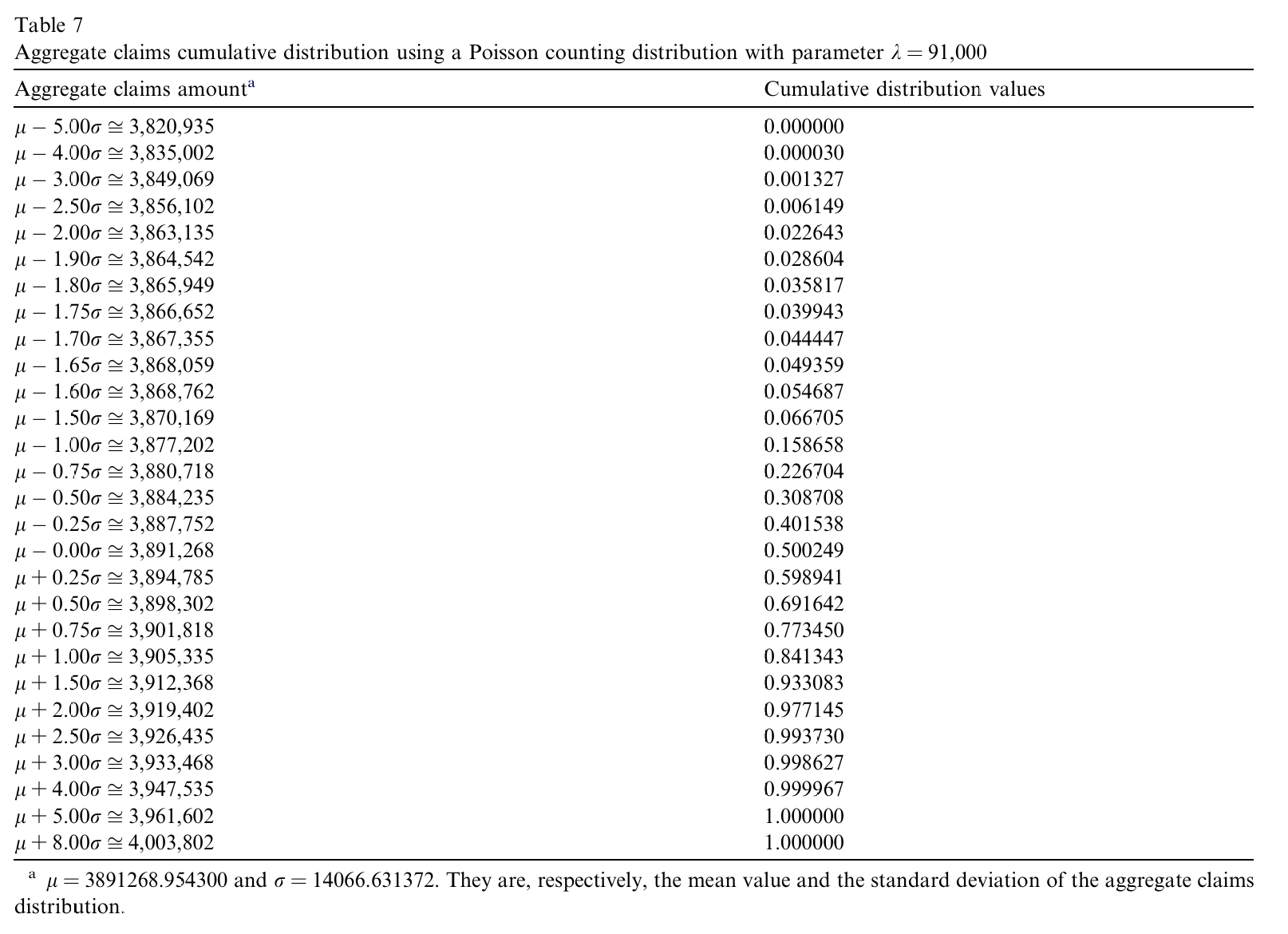
That is why the reproduction runs in seconds rather than hours, and why the ratio to their reported time is four orders of magnitude rather than the factor of 40 they anticipated in the other direction. Some of the gap is twenty years of hardware. The structural part is not.

6.2 What survives, and it is not nothing

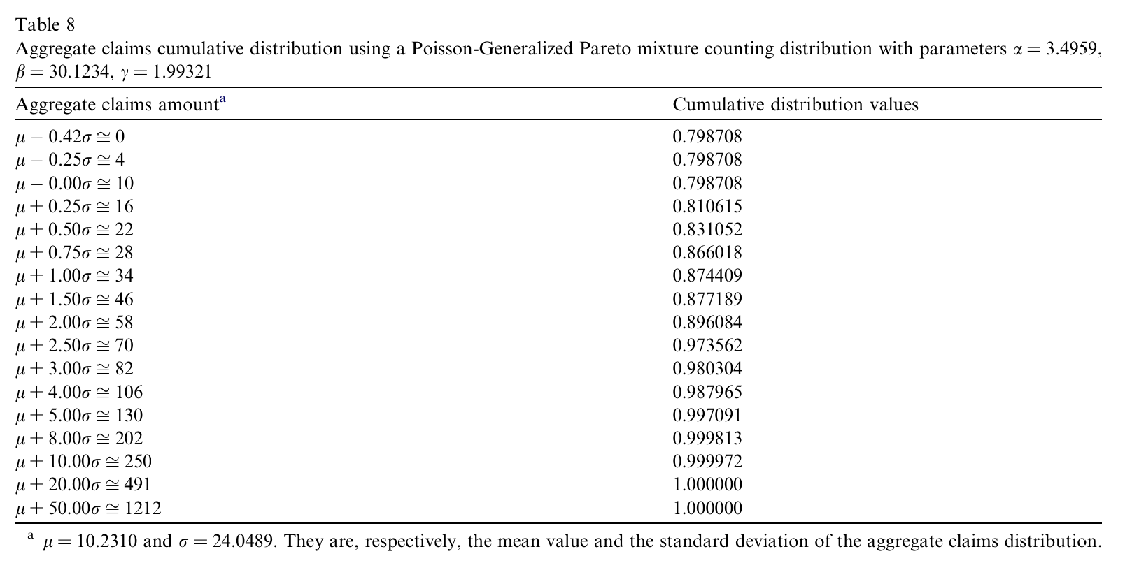
The threshold idea is sound and aggregate uses a version of it. Table 8 needed the frequency vector only out to \(n = 17\), because \(p(n)\) had fallen below \(10^{-14}\) by then, and that truncation is exactly the paper’s first phase. Their control, choosing the cutoff so that the retained mass and the first three moments are accurate to a stated tolerance, rather than by eye, is a good discipline and the closest thing in the paper to a genuinely portable idea. aggregate’s validation reports the analogous quantity as a moment comparison after the fact.

The underflow point also survives. Panjer recursion really does fail at \(\lambda = 1004.8\) here while the transform does not, and that is a real structural difference between recursions that propagate a small \(g(0)\) and methods that do not. It just happens to be an argument for the FFT rather than against it.

6.3 The severity is the interesting part

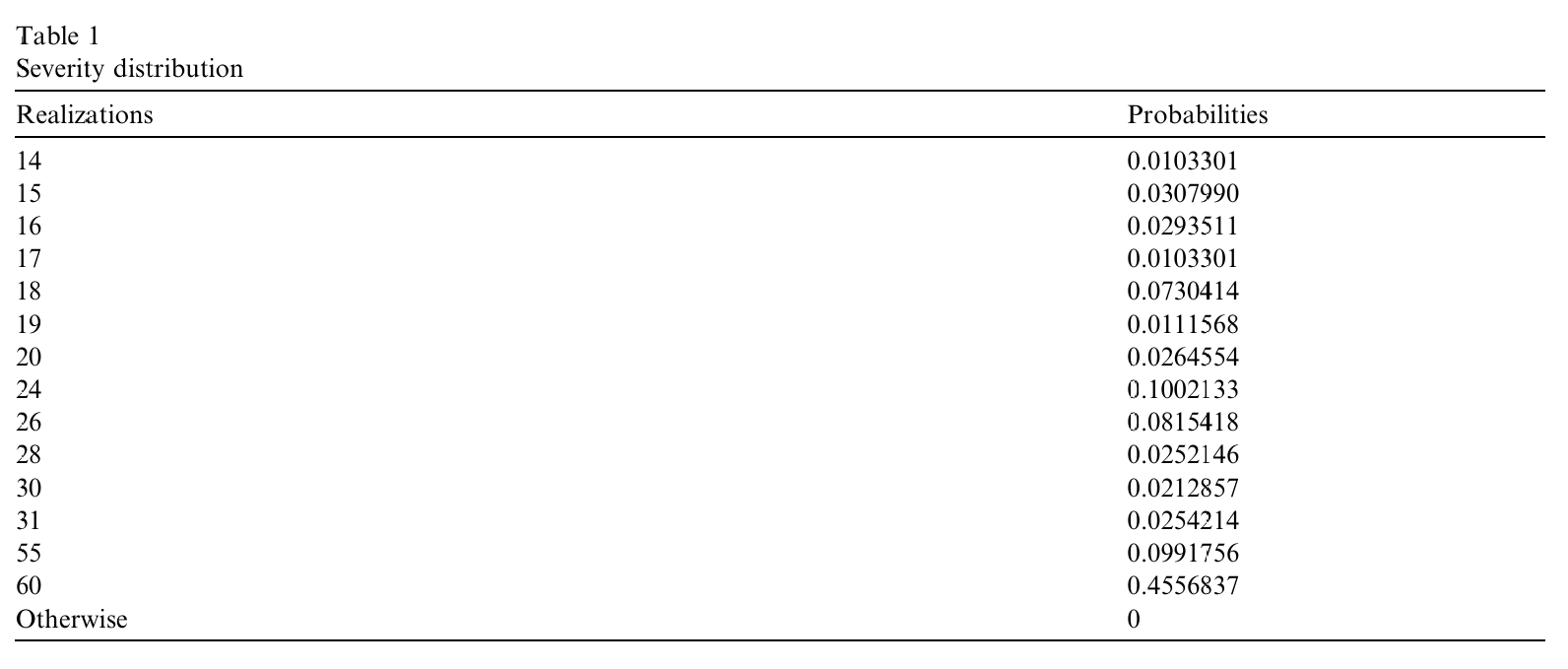
The 14-point severity carries 45.6% of its mass at the single value 60 and another 9.9% at 55, so more than half the distribution sits on two atoms at the top of the range. That is what makes the case a fair stress test: the aggregate is a convolution of a very lumpy lattice law, and a method that smoothed it would show up immediately. Both the paper’s method and aggregate reproduce the probability column, not just the CDF, which is the stronger test of the two.

Programs in the aggregate Loss Lab

Each program below opens in the aggregate Loss Lab, which builds it with nothing to install. The names are those in reproductions.agg, where every program is renamed by its paper’s citation key.

• Bruno2006.B: Table 6's compound Poisson at the smaller lambda.
• Bruno2006.B8: Table 8's model, with the frequency given as a discrete law.
• Bruno2006.B7: Table 7's compound Poisson at lambda = 91,000.

Bruno, M. G., Camerini, E., Manna, A., & Tomassetti, A. (2006). A new method for evaluating the distribution of aggregate claims. Applied Mathematics and Computation. https://doi.org/10.1016/j.amc.2005.09.038