Bear and Nemlick on adjustable treaty features

Reproducing Bear and Nemlick (1990), Table I

Author

Stephen J. Mildenhall

Published

2026-10-22 19:55 commit b5ca906+

1 Context and problem

An excess of loss treaty is rarely a flat exchange of premium for cover. It carries provisions that make the money depend on the loss: an annual aggregate deductible, a limited number of reinstatements, a loss corridor the cedant takes back, a retrospective rating plan on the premium, a profit commission, a sliding scale commission. Bear and Nemlick (1990) is the standard treatment of the family, and its organizing observation is that all six are the same object. Each is a deterministic function of a realized loss quantity, so each is priced by pushing that function forward over the aggregate loss distribution. Nothing about the treaty changes except which line of the statement the function writes into.

That reduces pricing to one question: where does the aggregate loss distribution come from? The paper answers it twice. The lognormal model fits a lognormal to the aggregate mean and coefficient of variation and reads the answer out of a printed table of excess pure premium ratios. The collective risk model builds the distribution properly, by characteristic function inversion, using the Heckman-Meyers algorithm. The paper’s purpose is to find out how much the cheap method costs, and its conclusion is that for these six treaties it costs very little.

Both models are what aggregate computes directly, and the six features are now six DecL clauses. This page reproduces the paper’s Table I: the lognormal column by rebuilding the paper’s own arithmetic, and the collective risk column by FFT. Table 1 is the whole mapping.

Table 1: The six adjustable features and the DecL clause that carries each.

Treaty	Feature	The clause
I	aggregate deductible	`aggregate net of 360 xs 0`
II	three free reinstatements	`occurrence net of 700 xs 0 deposit 1172 reinstatements 3 free`
III	loss corridor	`corridor 100% po 100% xs 100%`
IV	retrospective rating	`retro basic 0 lcm 1.3333 min 360 max 1200 premium`
V	profit commission	`pc 25% after 20%`
VI	sliding scale commission	`slide 40% at 35% and 25% at 55% and 20% at 65%`

2 Paper solution and gold standard

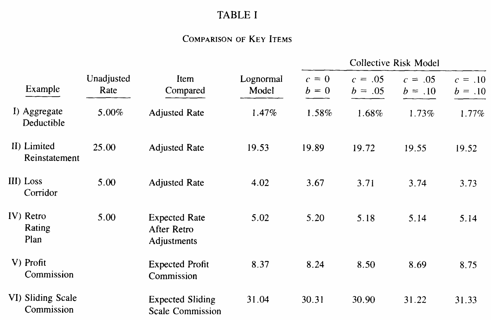
Table I on page 75, Figure 6, is the target. It gives, for each treaty, the item the feature is priced for, under the lognormal model and under four runs of the collective risk model indexed by a contagion parameter $c$ and a mixing parameter $b$. Table 2 transcribes it.

Table 2: Bear and Nemlick (1990), Table I as printed.

Example	Unadjusted rate	Item compared	Lognormal	$c=0$, $b=0$	$c=.05$, $b=.05$	$c=.05$, $b=.10$	$c=.10$, $b=.10$
I Aggregate deductible	5.00%	adjusted rate	1.47%	1.58	1.68	1.73	1.77
II Limited reinstatement	25.00	adjusted rate	19.53	19.89	19.72	19.55	19.52
III Loss corridor	5.00	adjusted rate	4.02	3.67	3.71	3.74	3.73
IV Retro rating plan	5.00	expected rate after retro	5.02	5.20	5.18	5.14	5.14
V Profit commission		expected profit commission	8.37	8.24	8.50	8.69	8.75
VI Sliding scale commission		expected sliding scale commission	31.04	30.31	30.90	31.22	31.33

The two parameters are Heckman-Meyers uncertainty loadings. Appendix C defines $c$ as the variance of a gamma variable with mean one multiplying the Poisson claim count mean, which is exactly aggregate’s gamma mixed Poisson: DecL mixed gamma {sqrt(c)}, since the clause takes the coefficient of variation of a mixing distribution whose mean is one. It defines $b$ as the variance of an inverse gamma variable with mean one dividing the severity. There is no analog of $b$ in DecL, so only the $c=0$, $b=0$ column is a like for like comparison. The other three are shown throughout, and the contagion only counterpart beside them.

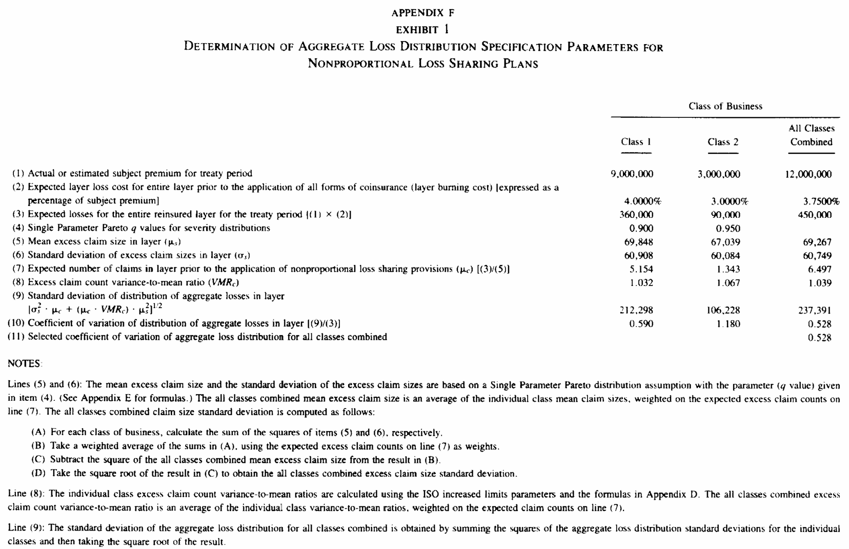
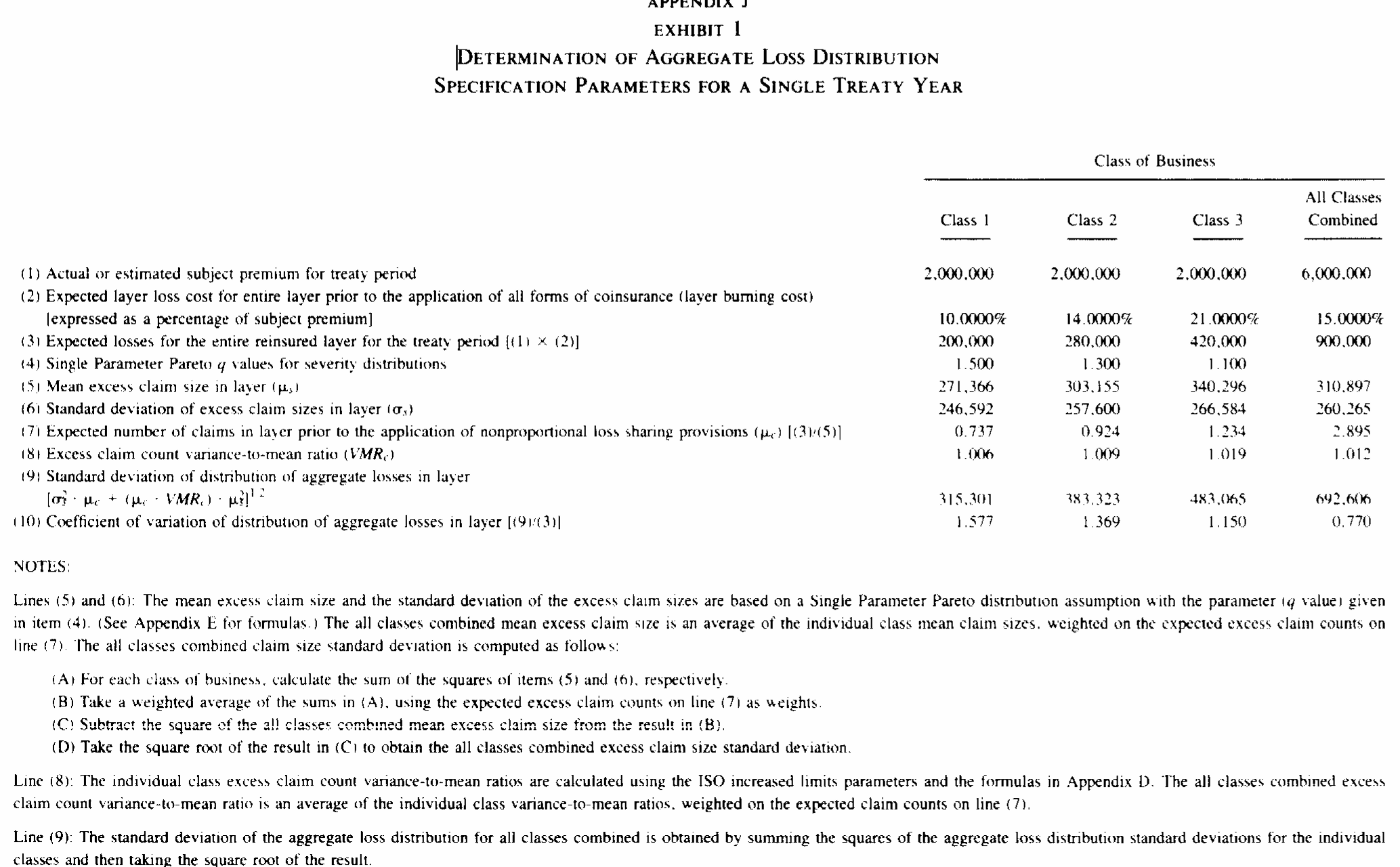
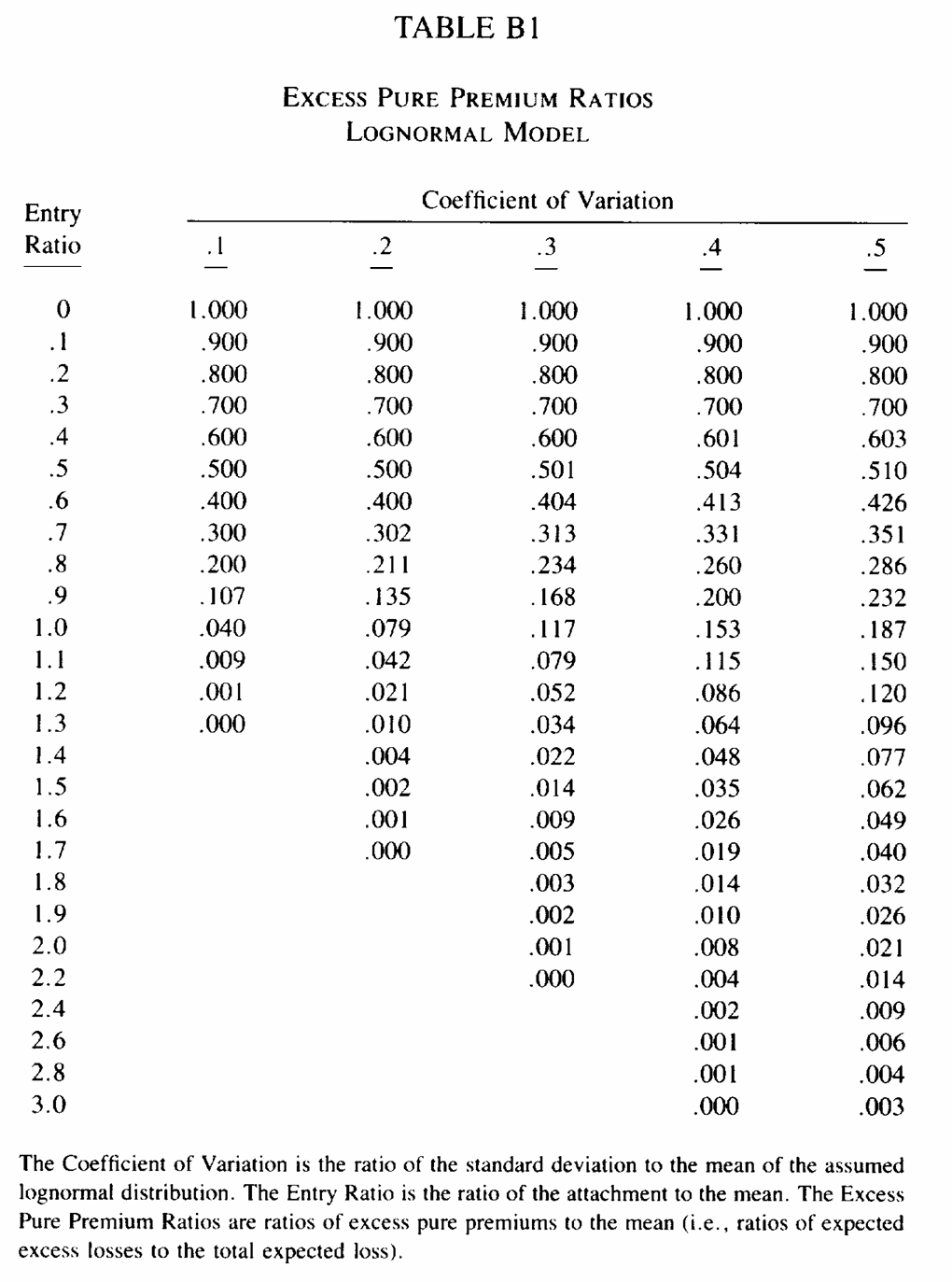
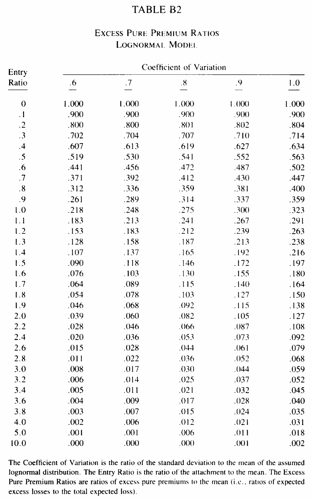
Two more exhibits are needed, and both are reproducible in their own right. Appendix F Exhibit 1 and Appendix J Exhibit 1, Figure 1 and Figure 2, derive the aggregate coefficient of variation for the two subject books from a single parameter Pareto severity and an excess claim count variance to mean ratio. Appendix B prints the lognormal excess pure premium ratio tables the whole lognormal method reads from.

2.1 The two subject books

All amounts on this page are in $000.

Treaties I and IV sit on the same book: $160 excess of $40 per occurrence, subject premium $12,000 split $9,000 and $3,000 between two classes with layer loss costs of 4.00% and 3.00% of subject premium, and single parameter Pareto severity with shape $q$ of 0.90 and 0.95.

Treaties II and V sit on the other: $700 excess of $300 per occurrence, subject premium $6,000 split equally between three classes with layer loss costs of 10%, 14% and 21%, and Pareto shapes 1.5, 1.3 and 1.1. Treaty V runs the same book for three years.

Treaty III is $400 excess of $100 on $10,000 of subject premium in three classes at 3.20%, 3.80% and 3.50%, all with $q = 1.1$. Treaty VI is $900 excess of $100 on $25,000 of subject premium, and the paper gives nothing about it beyond a 10% layer loss cost and a coefficient of variation of 0.485.

The single parameter Pareto with truncation $k$ and shape $q$ has $S(w) = (k/w)^q$ on $w \ge k$, so a loss excess of $k$ is a two parameter Pareto with scale $k$ and shape $q$: DecL {k} * pareto {q} - {k}, supported on $[0, \infty)$. Layered at the treaty limit it gives the excess claim size distribution Figure 1 and Figure 2 tabulate.

%xmode minimal
import warnings

import numpy as np
import pandas as pd
from aggregate import lognorm_fit, lognorm_lev
from bookstyle import GT, build

# Treaty II cedes its whole severity, so the net severity is a point mass at
# zero whose empirical variance lands a rounding below it and trips numpy on
# the square root. Cosmetic, and it reaches nothing on this page.
warnings.filterwarnings('ignore', 'invalid value encountered in sqrt')


def mixing_cv(vmr, claims):
    """Gamma mixing CV giving an excess claim count variance to mean ratio.

    A gamma mixed Poisson with mixing CV c and mean n has variance
    n + n^2 c^2, so the variance to mean ratio is 1 + n c^2.
    """
    return float(np.sqrt((vmr - 1) / claims))


def exhibit_1(port, printed):
    """Compare a book's per class parameters with the paper's Exhibit 1."""
    rows = [{'class': a.name, 'claims': a.n, 'severity mean': a.sev_m,
             'severity sd': a.sev_m * a.sev_cv, 'aggregate mean': a.actual_m,
             'aggregate sd': a.actual_m * a.actual_cv,
             'aggregate cv': a.actual_cv} for a in port]
    rows.append({'class': 'all classes', 'claims': sum(a.n for a in port),
                 'severity mean': np.nan, 'severity sd': np.nan,
                 'aggregate mean': port.est_m,
                 'aggregate sd': port.est_m * port.est_cv,
                 'aggregate cv': port.est_cv})
    got = pd.DataFrame(rows).set_index('class')
    out = pd.concat({'aggregate': got, 'paper': printed.reindex(got.index)},
                    axis=1).swaplevel(axis=1).sort_index(axis=1)
    return out[got.columns]

Exception reporting mode: Minimal

Appendix F Exhibit 1, Figure 1, in full. The excess claim count variance to mean ratios in line 8 come from ISO increased limits parameters and are the paper’s own inputs, so they are given to the build rather than derived. Table 3 is the comparison.

Figure 1: Bear and Nemlick (1990), Appendix F, Exhibit 1.

book_1 = build(f'''
port BearNemlick.One
    agg Class1 9000 exposure at 0.04 rate 160 xs 0
        sev 40 * pareto 0.90 - 40 mixed gamma {mixing_cv(1.032, 5.154)}
    agg Class2 3000 exposure at 0.03 rate 160 xs 0
        sev 40 * pareto 0.95 - 40 mixed gamma {mixing_cv(1.067, 1.343)}
''')

printed_1 = pd.DataFrame(
    [[5.154, 69_848, 60_908, 360_000, 212_298, 0.590],
     [1.343, 67_039, 60_084,  90_000, 106_228, 1.180],
     [6.497, np.nan, np.nan, 450_000, 237_391, 0.528]],
    index=['Class1', 'Class2', 'all classes'],
    columns=['claims', 'severity mean', 'severity sd', 'aggregate mean',
             'aggregate sd', 'aggregate cv']) / [1, 1e3, 1e3, 1e3, 1e3, 1]
GT(exhibit_1(book_1, printed_1), float_format=3)

Table 3: The first subject book, class by class, against Appendix F Exhibit 1.

	claims		severity mean		severity sd		aggregate mean		aggregate sd		aggregate cv
class	aggregate	paper	aggregate	paper	aggregate	paper	aggregate	paper	aggregate	paper	aggregate	paper
Class1	5.154	5.154	69.848	69.848	60.908	60.908	360.000	360	212.298	212.298	0.590	0.590
Class2	1.343	1.343	67.039	67.039	60.084	60.084	90.000	90	106.227	106.228	1.180	1.180
all classes	6.497	6.497	—	—	—	—	450.000	450	237.391	237.391	0.528	0.528

Appendix J Exhibit 1, Figure 2, the same for the second book, compared in Table 4.

Figure 2: Bear and Nemlick (1990), Appendix J, Exhibit 1.

book_2 = build(f'''
port BearNemlick.Two
    agg Class1 2000 exposure at 0.10 rate 700 xs 0
        sev 300 * pareto 1.5 - 300 mixed gamma {mixing_cv(1.006, 0.737)}
    agg Class2 2000 exposure at 0.14 rate 700 xs 0
        sev 300 * pareto 1.3 - 300 mixed gamma {mixing_cv(1.009, 0.924)}
    agg Class3 2000 exposure at 0.21 rate 700 xs 0
        sev 300 * pareto 1.1 - 300 mixed gamma {mixing_cv(1.019, 1.234)}
''')

printed_2 = pd.DataFrame(
    [[0.737, 271_395, 246_596, 200_000, 315_301, 1.577],
     [0.924, 303_133, 257_600, 280_000, 383_323, 1.369],
     [1.234, 340_296, 266_584, 420_000, 483_065, 1.150],
     [2.895, np.nan, np.nan, 900_000, 692_606, 0.770]],
    index=['Class1', 'Class2', 'Class3', 'all classes'],
    columns=['claims', 'severity mean', 'severity sd', 'aggregate mean',
             'aggregate sd', 'aggregate cv']) / [1, 1e3, 1e3, 1e3, 1e3, 1]
GT(exhibit_1(book_2, printed_2), float_format=3)

Table 4: The second subject book, class by class, against Appendix J Exhibit 1.

	claims		severity mean		severity sd		aggregate mean		aggregate sd		aggregate cv
class	aggregate	paper	aggregate	paper	aggregate	paper	aggregate	paper	aggregate	paper	aggregate	paper
Class1	0.737	0.737	271.366	271.395	246.592	246.596	200.000	200	315.301	315.301	1.577	1.577
Class2	0.924	0.924	303.155	303.133	257.600	257.600	280.000	280	383.323	383.323	1.369	1.369
Class3	1.234	1.234	340.296	340.296	266.584	266.584	420.000	420	483.066	483.065	1.150	1.150
all classes	2.895	2.895	—	—	—	—	900.000	900	692.606	692.606	0.770	0.770

Across Table 3 and Table 4, every claim count, every excess claim size moment and every aggregate standard deviation comes back at the paper’s printed precision, and with it the two coefficients of variation the lognormal method needs, 0.528 and 0.770. The two severity means in the second book differ in the fifth figure, 271.37 against 271.395 and 303.15 against 303.133, which is rounding in Appendix J Exhibit 1 rather than a difference of model.

2.2 The lognormal tables

The lognormal method needs the excess pure premium ratio $P_2(r)$, the expected loss above an attachment at entry ratio $r$ divided by the expected loss, for a unit mean lognormal with a given coefficient of variation. The paper prints it in Tables B1 to B3, Figure 3 and Figure 4, and interpolates linearly in both arguments. Reproducing Table I therefore means reproducing the interpolation, not the exact lognormal: the two differ by up to seven basis points at the entry ratios these treaties use, which is enough to move a printed answer. Table 5 checks the transcribed cells.

Figure 3: Bear and Nemlick (1990), Appendix B, Table B1.

Figure 4: Bear and Nemlick (1990), Appendix B, Table B2.

# The cells of Tables B1 and B2 the six exhibits reach into, printed excess pure
# premium ratio by entry ratio then coefficient of variation.
B = {
    0.0: {0.4: 1.000, 0.5: 1.000},
    0.6: {0.5: 0.426, 0.6: 0.441},
    0.7: {0.4: 0.331, 0.5: 0.351},
    0.8: {0.5: 0.286, 0.6: 0.312},
    1.0: {0.9: 0.300, 1.0: 0.323},
    1.1: {0.4: 0.115, 0.5: 0.150},
    1.3: {0.4: 0.064, 0.5: 0.096},
    1.6: {0.4: 0.026, 0.5: 0.049},
    1.7: {0.4: 0.019, 0.5: 0.040},
    2.0: {0.5: 0.021, 0.6: 0.039, 0.9: 0.105, 1.0: 0.127},
    3.0: {0.7: 0.017, 0.8: 0.030},
    3.2: {0.7: 0.014, 0.8: 0.025},
}


def _interp(row, cv):
    lo, hi = max(c for c in row if c <= cv), min(c for c in row if c >= cv)
    if lo == hi:
        return row[lo]
    return row[lo] + (cv - lo) / (hi - lo) * (row[hi] - row[lo])


def charge(cv, r):
    """Insurance charge P2(r), by linear interpolation in Tables B1 to B3."""
    lo = max(x for x in B if x <= r)
    hi = min(x for x in B if x >= r)
    if lo == hi:
        return _interp(B[lo], cv)
    a, b = _interp(B[lo], cv), _interp(B[hi], cv)
    return a + (r - lo) / (hi - lo) * (b - a)


def exact_charge(cv, r):
    """P2(r) for the lognormal itself, with no table in the way."""
    if r == 0:
        return 1.0
    mu, sigma = lognorm_fit(1, cv)
    return 1 - lognorm_lev(mu, sigma, 1, r)


cells = pd.DataFrame([{'entry ratio': r, 'cv': cv, 'printed': v,
                       'exact lognormal': exact_charge(cv, r),
                       'difference': v - exact_charge(cv, r)}
                      for r, row in sorted(B.items()) for cv, v in sorted(row.items())])
GT(cells, float_format=5)

Table 5: Every cell of Tables B1 and B2 the six exhibits reach into, against the exact lognormal.

entry ratio	cv	printed	exact lognormal	difference
0.00000	0.40000	1.00000	1.00000	0.00000
0.00000	0.50000	1.00000	1.00000	0.00000
0.60000	0.50000	0.42600	0.42558	0.00042
0.60000	0.60000	0.44100	0.44051	0.00049
0.70000	0.40000	0.33100	0.33052	0.00048
0.70000	0.50000	0.35100	0.35057	0.00043
0.80000	0.50000	0.28600	0.28602	-0.00002
0.80000	0.60000	0.31200	0.31180	0.00020
1.00000	0.90000	0.30000	0.29987	0.00013
1.00000	1.00000	0.32300	0.32279	0.00021
1.10000	0.40000	0.11500	0.11520	-0.00020
1.10000	0.50000	0.15000	0.14995	0.00005
1.30000	0.40000	0.06400	0.06413	-0.00013
1.30000	0.50000	0.09600	0.09619	-0.00019
1.60000	0.40000	0.02600	0.02591	0.00009
1.60000	0.50000	0.04900	0.04938	-0.00038
1.70000	0.40000	0.01900	0.01911	-0.00011
1.70000	0.50000	0.04000	0.03962	0.00038
2.00000	0.50000	0.02100	0.02066	0.00034
2.00000	0.60000	0.03900	0.03864	0.00036
2.00000	0.90000	0.10500	0.10458	0.00042
2.00000	1.00000	0.12700	0.12688	0.00012
3.00000	0.70000	0.01700	0.01748	-0.00048
3.00000	0.80000	0.03000	0.02958	0.00042
3.20000	0.70000	0.01400	0.01396	0.00004
3.20000	0.80000	0.02500	0.02458	0.00042

In Table 5 no transcribed cell is more than 5 in the fourth decimal from the exact lognormal, which is the rounding of a three decimal table, so the transcription is sound and the B tables are what they claim to be.

3 The `aggregate` reproduction

Each treaty is one program. The subject book is an agg, the feature is a clause on it, and the answer is a mean read off the resulting PnL. Every treaty is built at all three contagion levels, so the functions below take the frequency clause as an argument.

Five of the six use xpnl, the walk face, which books each cession as its own step and so gives the ceded recovery, the ceded premium and any commission as separate legs. Treaty IV uses pnl, the consolidated net view, because a retro plan varies the gross premium and there is no cession to walk.

FREQ = {'c = 0': 'poisson',
        'c = .05': 'mixed gamma 0.05**0.5',
        'c = .10': 'mixed gamma 0.1**0.5'}


def leg(pnl, label):
    """One ledger leg's expected value, off the PnL's own economic_df."""
    return float(pnl.economic_df.xs(label, level='Label').iloc[0]['EX'])

3.1 Treaty I: aggregate deductible

The treaty carries an annual aggregate deductible of 3% of subject premium, $360 against $450 of expected layer loss, an entry ratio of 0.800. The rate is the loss cost surviving the deductible, loaded 100/75.

An aggregate deductible is an aggregate layer the cedant keeps, so the recovery is the aggregate net of it. Table 6 prices it.

BOOK_1 = ('agg BN.One [9000 3000] exposure at [0.04 0.03] rate 160 xs 0 '
          'sev 40 * pareto [0.90 0.95] - 40 {freq} ')


def treaty_1(freq):
    gross = build(BOOK_1.format(freq=freq))
    net = build(BOOK_1.format(freq=freq) + 'aggregate net of 360 xs 0')
    return {'cv': gross.actual_cv, 'charge': net.est_m / gross.actual_m,
            'key': 100 / 75 * 3.75 * net.est_m / gross.actual_m}


one = treaty_1(FREQ['c = 0'])
GT(pd.DataFrame([{'insurance charge, aggregate': one['charge'],
                  'insurance charge, lognormal': charge(0.528, 360 / 450),
                  'adjusted rate %, aggregate': one['key'],
                  'adjusted rate %, paper c = 0': 1.58,
                  'adjusted rate %, paper lognormal': 1.47}]), float_format=4)

Table 6: Treaty I, the insurance charge and adjusted rate under both models, against Table I.

insurance charge, aggregate	insurance charge, lognormal	adjusted rate %, aggregate	adjusted rate %, paper c = 0	adjusted rate %, paper lognormal
0.3151	0.2933	1.5755	1.5800	1.4700

The paper’s Appendix F Exhibit 2 puts the insurance charge at 29.33% and the indicated rate at 1.4664%, against 1.47% printed in Table I. In Table 6 the exact distribution puts the charge two and a fifth points higher, which is the whole story of the treaty: the lognormal fitted to a mean of 450 and a coefficient of variation of 0.528 is more skewed than the real aggregate, so it leaves too little mass in the body and overstates what a deductible at 0.8 times the mean eliminates.

3.2 Treaty II: three free reinstatements

Three free reinstatements plus the original limit give total annual capacity of $4 \times 700 = 2800$, against $900 of expected layer loss, an entry ratio of 3.111. Then 20% of layer losses are coinsured without a share of premium, and the result is loaded 100/60.

This is where the reinstatement clause earns its place. The treaty language is three free reinstatements, and that is what goes in the program. The annual cap follows from it rather than being computed by hand and entered as an aggregate limit.

The schedule needs a base premium to price reinstatements against, and the deposit of $1,172 is the paper’s own indicated treaty premium, 19.53% of $6,000. Free reinstatements charge nothing, so it does not reach the recovery. Table 7 is the resulting ledger.

BOOK_2 = ('agg BN.Two [2000 2000 2000] exposure at [0.10 0.14 0.21] rate 700 xs 0 '
          'sev 300 * pareto [1.5 1.3 1.1] - 300 '
          'occurrence net of 700 xs 0 deposit 1172 reinstatements 3 free '
          'as "Layer" {freq} ')


def treaty_2(freq):
    x = build('xpnl BN.TreatyII 1172 premium less ' + BOOK_2.format(freq=freq))
    recovery = leg(x, 'Layer recovery')
    composite = 1 - 0.80 * recovery / x.engine.actual_m
    return {'cv': x.engine.actual_cv, 'recovery': recovery,
            'charge': 1 - recovery / x.engine.actual_m,
            'key': 100 / 60 * 15 * (1 - composite), 'x': x}


two = treaty_2(FREQ['c = 0'])
print(two['x'].engine.reinstatement_terms)

ReinstatementTerms(limit=700, rates=(0.0, 0.0, 0.0), deposit=1172, rol=1.674, m=3, Y=2800)

GT(two['x'].economic_df[['EX', 'SD', 'CV']], float_format=3)

Table 7: Treaty II, the P&L legs of the layer with three free reinstatements.

Step	Side	Label	EX	SD	CV
Gross	Consideration	Premium	1,172.000	0.000	0.000
	Obligation	Loss	-900.000	689.879	-0.767
	Margin	Gross	272.000	689.879	2.536
Layer	Consideration	Layer premium	-1,172.000	0.000	0.000
	Obligation	Layer recovery	894.878	672.732	0.752
	Margin	Total	-277.122	672.732	-2.428
	Margin	Net	-5.122	62.576	-12.218
All	Consideration	Net	0.000	0.000	—
	Obligation	Net	-5.122	62.576	-12.218
	Margin	Net	-5.122	62.576	-12.218
	Margin	Impact	-277.122	672.732	-2.428

The severity is already the loss to the layer, so the occurrence clause 700 xs 0 is the identity on each claim and the reinstatement schedule supplies the only binding term, the annual cap. The paper’s own reading of the same provision is an aggregate limit of 2800, and Table 8 shows the two agree.

alt = build('agg BN.TwoAlt [2000 2000 2000] exposure at [0.10 0.14 0.21] rate '
            '700 xs 0 sev 300 * pareto [1.5 1.3 1.1] - 300 poisson '
            'aggregate ceded to 2800 xs 0')
GT(pd.DataFrame([{'reinstatements 3 free': two['recovery'],
                  'aggregate ceded to 2800 xs 0': alt.est_m,
                  'relative difference': abs(two['recovery'] / alt.est_m - 1),
                  'insurance charge, aggregate': two['charge'],
                  'insurance charge, lognormal': charge(0.770, 2800 / 900),
                  'adjusted rate %, aggregate': two['key'],
                  'adjusted rate %, paper c = 0': 19.89}]), float_format=6)

Table 8: Treaty II, the reinstatement schedule against the equivalent aggregate limit, and the adjusted rate under both models.

reinstatements 3 free	aggregate ceded to 2800 xs 0	relative difference	insurance charge, aggregate	insurance charge, lognormal	adjusted rate %, aggregate	adjusted rate %, paper c = 0
894.878258	894.880498	0.000003	0.005691	0.023656	19.886184	19.890000

3.3 Treaty III: loss corridor

The reinsurer stops paying once layer losses reach 100% of expected and resumes above 200%. Expressed as entry ratios the band is one mean wide attaching at one mean, and the cedant takes all of it. Writing the base ceded premium as the expected layer loss of $350 makes the ceded loss ratio the entry ratio, so the corridor clause reads exactly as the slip does.

A corridor decorates an aggregate layer, and here the whole aggregate is ceded, so the layer is $10,000 excess of nothing: a limit far above anything the aggregate reaches, present only to give the corridor something to sit on. Table 9 prices it.

BOOK_3 = ('agg BN.Three [4500 4500 1000] exposure at [0.032 0.038 0.035] rate '
          '400 xs 0 sev 100 * pareto 1.1 - 100 {freq} '
          'aggregate net of 10000 xs 0 deposit 350 '
          'corridor 100% po 100% xs 100% as "Corridor" ')


def treaty_3(freq):
    x = build('xpnl BN.TreatyIII 10000 premium less ' + BOOK_3.format(freq=freq))
    recovery = leg(x, 'Corridor recovery')
    return {'cv': x.engine.actual_cv, 'recovery': recovery,
            'eliminated': 1 - recovery / 350,
            'key': 100 / 70 * 100 * recovery / 10000}


three = treaty_3(FREQ['c = 0'])
GT(pd.DataFrame([{
    'expected layer loss': 350.0,
    'after corridor, aggregate': three['recovery'],
    'eliminated, aggregate': three['eliminated'],
    'eliminated, lognormal': charge(0.905, 1.0) - charge(0.905, 2.0),
    'adjusted rate %, aggregate': three['key'],
    'adjusted rate %, paper c = 0': 3.67}]), float_format=4)

Table 9: Treaty III, the loss eliminated by the corridor under both models, and the adjusted rate against Table I.

expected layer loss	after corridor, aggregate	eliminated, aggregate	eliminated, lognormal	adjusted rate %, aggregate	adjusted rate %, paper c = 0
350	256.8761	0.2661	0.1950	3.6697	3.6700

The corridor reads a loss ratio, so its parameterization depends on what the ceded premium is called. Restating the same band against the indicated treaty premium, which is a different number, has to give the same recovery, and in Table 10 it does.

premium = 100 / 70 * three['recovery']
band = 350 / premium
restated = build(
    f'xpnl BN.TreatyIIIb 10000 premium less '
    + BOOK_3.format(freq=FREQ['c = 0'])
    .replace('deposit 350', f'deposit {premium}')
    .replace('po 100% xs 100%', f'po {band} xs {band}'))
GT(pd.DataFrame([{'indicated treaty premium': premium,
                  'band in loss ratio points': band,
                  'recovery, expected loss basis': three['recovery'],
                  'recovery, premium basis': leg(restated, 'Corridor recovery')}]),
   float_format=6)

Table 10: Treaty III’s corridor recovery on an expected loss basis and on a premium basis, which must agree.

indicated treaty premium	band in loss ratio points	recovery, expected loss basis	recovery, premium basis
366.965864	0.953767	256.876105	256.876105

3.4 Treaty IV: retrospective rating

The same book as Treaty I, flat rated at 5%, with a one year retro plan: the adjusted premium is 100/75 times incurred layer loss, subject to a maximum of 10% and a minimum of 3% of $12,000 subject premium. There is no basic premium and no flat margin, so the collar is the whole plan.

Retro varies the account premium rather than a cession, so in DecL it replaces the fixed premium at the head of the program. Table 11 is the resulting ledger.

def treaty_4(freq):
    p = build('pnl BN.TreatyIV '
              'retro basic 0 lcm 1.3333333333 min 360 max 1200 premium '
              'less ' + BOOK_1.format(freq=freq).replace('BN.One', 'BN.Four'))
    return {'cv': p.engine.actual_cv, 'premium': leg(p, 'Premium'),
            'key': 100 * leg(p, 'Premium') / 12000, 'p': p}


four = treaty_4(FREQ['c = 0'])
GT(four['p'].economic_df[['EX', 'SD', 'CV']], float_format=3)

Table 11: Treaty IV, the P&L legs under the retrospective rating plan.

Side	Label	EX	SD	CV
Consideration	Premium	624.510	253.880	0.407
Obligation	Loss	-450.000	234.831	-0.522
Margin	Total	174.510	62.482	0.358

In Table 11 the premium leg is now a distribution with a standard deviation, which is the point of a retro plan, and its mean divided by subject premium is the expected rate after all retro adjustments, in Table 12.

r_max, r_min = (10 / (100 / 75)) / 3.75, (3 / (100 / 75)) / 3.75
net_charge = charge(0.528, r_max) - (r_min + charge(0.528, r_min) - 1)
GT(pd.DataFrame([{
    'entry ratio at maximum': r_max, 'entry ratio at minimum': r_min,
    'net insurance charge, lognormal': net_charge,
    'expected rate %, lognormal': 100 / 75 * 3.75 * (1 - net_charge),
    'expected rate %, aggregate': four['key'],
    'expected rate %, paper c = 0': 5.20,
    'off balance factor, aggregate': 5.0 / four['key']}]), float_format=4)

Table 12: Treaty IV, the collar as entry ratios, the net insurance charge, and the expected rate after retro under both models.

entry ratio at maximum	entry ratio at minimum	net insurance charge, lognormal	expected rate %, lognormal	expected rate %, aggregate	expected rate %, paper c = 0	off balance factor, aggregate
2	0.6000	-0.0042	5.0208	5.2042	5.2000	0.9608

3.5 Treaty V: three year profit commission

The second book run for three years, $18,000 of subject premium, treaty rate 25%, so $4,500 of treaty premium against $2,700 of expected layer loss. A 20% coinsurance leaves the reinsurer with $2,160, an expected ceded loss ratio of 48%. The profit commission returns 25% of the reinsurer’s profit after a 20% overhead allowance, a put on the ceded loss ratio struck at 80%.

The coinsurance is a share of the loss with no corresponding share of premium. In DecL that is a placement: premium clauses are quoted at 100% and scaled by the fraction placed, so a slip premium of $4,500 on an 80% placement is a deposit of $5,625. The layer it is placed on is again nominal, wide enough to reach everything the three year aggregate does. Table 13 is the resulting ledger.

BOOK_5 = ('agg BN.Five [6000 6000 6000] exposure at [0.10 0.14 0.21] rate '
          '700 xs 0 sev 300 * pareto [1.5 1.3 1.1] - 300 {freq} '
          'aggregate net of 80% po 100000 xs 0 deposit 5625 '
          'pc 25% after 20% as "PC layer" ')


def treaty_5(freq):
    x = build('xpnl BN.TreatyV 18000 premium less ' + BOOK_5.format(freq=freq))
    return {'cv': x.engine.actual_cv, 'pc': leg(x, 'profit commission'),
            'key': 100 * leg(x, 'profit commission') / 4500, 'x': x}


five = treaty_5(FREQ['c = 0'])
GT(five['x'].economic_df[['EX', 'SD', 'CV']], float_format=3)

Table 13: Treaty V, the P&L legs of the three year book carrying the profit commission.

Step	Side	Label	EX	SD	CV
Gross	Consideration	Premium	18,000.000	0.000	0.000
	Obligation	Loss	-2,700.000	1,194.862	-0.443
	Margin	Gross	15,300.000	1,194.862	0.078
PC layer	Consideration	PC layer premium	-4,500.000	0.000	0.000
	Obligation	PC layer recovery	2,160.000	955.889	0.443
		profit commission	370.725	215.746	0.582
		Total	2,530.725	745.716	0.295
	Margin	Total	-1,969.275	745.716	-0.379
	Margin	Net	13,330.725	452.437	0.034
All	Consideration	Net	13,500.000	0.000	0.000
	Obligation	Net	-169.275	452.437	-2.673
	Margin	Net	13,330.725	452.437	0.034
	Margin	Impact	-1,969.275	745.716	-0.379

elr = 0.15 * 0.80 / 0.25
GT(pd.DataFrame([{
    'expected ceded loss ratio': elr,
    'entry ratio at breakeven': 0.80 / elr,
    'net insurance charge, lognormal': charge(0.444, 0.80 / elr),
    'simplistic view %': 100 * 0.25 * (1 - elr - 0.20),
    'expected pc %, lognormal': 100 * 0.25 * (1 - elr * (1 - charge(0.444, 0.80 / elr)) - 0.20),
    'expected pc %, aggregate': five['key'],
    'expected pc %, paper c = 0': 8.24}]), float_format=4)

Table 14: Treaty V, the expected profit commission under both models and under the simplistic view, against Table I.

expected ceded loss ratio	entry ratio at breakeven	net insurance charge, lognormal	simplistic view %	expected pc %, lognormal	expected pc %, aggregate	expected pc %, paper c = 0
0.4800	1.6667	0.0309	8	8.3704	8.2383	8.2400

In Table 14 the simplistic view plugs the expected loss ratio into the formula and gets 8.00%. Both models return more, because the profit commission is a positive part and therefore convex, so its expected value exceeds its value at the mean. The paper calls the difference the actuarial view; it is Jensen’s inequality, and it is a property of the whole distribution rather than of any moment of it.

3.6 Treaty VI: sliding scale commission

$900 excess of $100 on $25,000 of subject premium, layer loss cost 10%, treaty rate 20%, so an expected treaty loss ratio of 50%. The commission is 20% at a loss ratio of 65% and above, slides up half a point per point down to 25% at 55%, then three quarters of a point per point up to 40% at 35%, and is flat at 40% below that. The plan is exactly the anchor form the slide clause takes.

Nothing else about the book is published, only its coefficient of variation of 0.485. The Pareto shape is therefore a free parameter, fixed here by solving for the value that reproduces the stated coefficient of variation under Poisson counts. Table 15 is the resulting ledger.

BOOK_6 = ('agg BN.Six 25000 exposure at 0.10 rate 900 xs 0 '
          'sev 100 * pareto {q} - 100 {freq} '
          'aggregate net of 100000 xs 0 deposit 5000 '
          'slide 40% at 35% and 25% at 55% and 20% at 65% as "Slide" ')
Q6 = 0.98


def treaty_6(freq, q=Q6):
    x = build('xpnl BN.TreatyVI 25000 premium less '
              + BOOK_6.format(freq=freq, q=q))
    return {'cv': x.engine.actual_cv, 'slide': leg(x, 'sliding commission'),
            'key': 100 * leg(x, 'sliding commission') / 5000, 'x': x}


six = treaty_6(FREQ['c = 0'])
GT(six['x'].economic_df[['EX', 'SD', 'CV']], float_format=3)

Table 15: Treaty VI, the P&L legs of the book carrying the sliding scale commission.

Step	Side	Label	EX	SD	CV
Gross	Consideration	Premium	25,000.000	0.000	0.000
	Obligation	Loss	-2,499.999	1,212.545	-0.485
	Margin	Gross	22,500.001	1,212.545	0.054
Slide	Consideration	Slide premium	-5,000.000	0.000	0.000
	Obligation	Slide recovery	2,499.999	1,212.545	0.485
		sliding commission	1,515.866	417.931	0.276
		Total	4,015.865	856.660	0.213
	Margin	Total	-984.135	856.660	-0.870
	Margin	Net	21,515.866	417.931	0.019
All	Consideration	Net	20,000.000	0.000	0.000
	Obligation	Net	1,515.866	417.931	0.276
	Margin	Net	21,515.866	417.931	0.019
	Margin	Impact	-984.135	856.660	-0.870

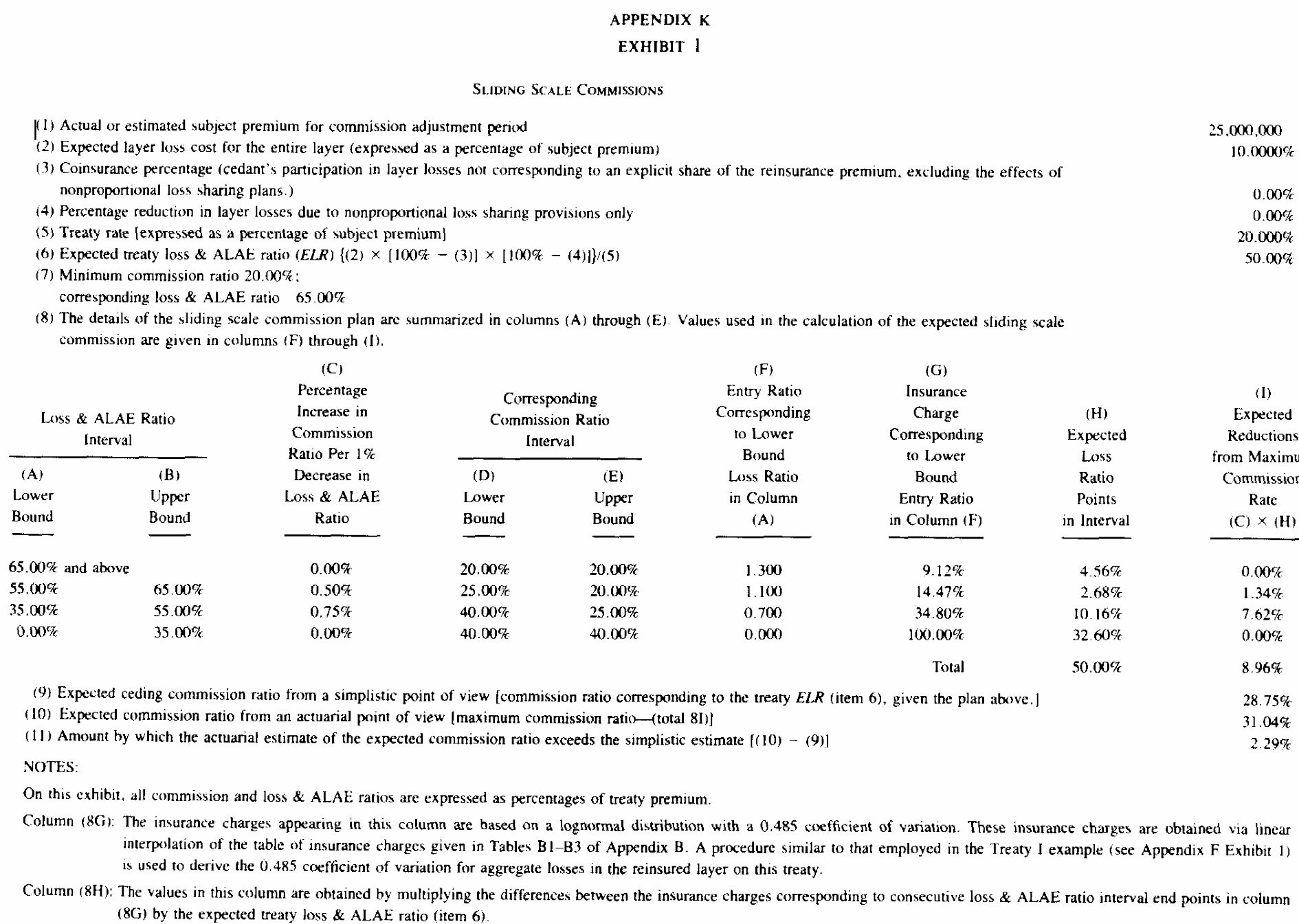
The paper’s own calculation walks the four loss ratio intervals, weights each by the expected loss ratio points falling in it, and subtracts the commission given up from the maximum. That is Appendix K Exhibit 1, Figure 5, and Table 16 reproduces it line by line.

Figure 5: Bear and Nemlick (1990), Appendix K, Exhibit 1.

SLIDE = [('65% and above', 0.65, 0.00, 0.20), ('55% to 65%', 0.55, 0.50, 0.25),
         ('35% to 55%', 0.35, 0.75, 0.40), ('0% to 35%', 0.00, 0.00, 0.40)]
elr6 = 0.10 / 0.20
rows, prev = [], 0.0
for band, lower, slope, commission in SLIDE:
    p2 = charge(0.485, lower / elr6)
    points = elr6 * (p2 - prev)
    rows.append({'loss ratio interval': band, 'commission': commission,
                 'slide per point': slope, 'entry ratio': lower / elr6,
                 'insurance charge': p2, 'loss ratio points': points,
                 'reduction from maximum': slope * points})
    prev = p2
k1 = pd.DataFrame(rows).set_index('loss ratio interval')
k1.loc['total'] = k1[['loss ratio points', 'reduction from maximum']].sum()
GT(k1, float_format=4)

Table 16: Appendix K Exhibit 1 rebuilt, the four loss ratio intervals and the commission given up in each.

loss ratio interval	commission	slide per point	entry ratio	insurance charge	loss ratio points	reduction from maximum
65% and above	0.2000	0.0000	1.3000	0.0912	0.0456	0.0000
55% to 65%	0.2500	0.5000	1.1000	0.1447	0.0268	0.0134
35% to 55%	0.4000	0.7500	0.7000	0.3480	0.1016	0.0762
0% to 35%	0.4000	0.0000	0.0000	1.0000	0.3260	0.0000
total	—	—	—	—	0.5000	0.0896

GT(pd.DataFrame([{
    'aggregate cv': six['cv'], 'paper cv': 0.485,
    'simplistic view %': 100 * (0.25 + 0.75 * (0.55 - elr6)),
    'expected commission %, lognormal': 100 * (0.40 - k1.loc['total', 'reduction from maximum']),
    'expected commission %, aggregate': six['key'],
    'expected commission %, paper c = 0': 30.31}]), float_format=4)

Table 17: Treaty VI, the expected sliding scale commission under both models and under the simplistic view, against Table I.

aggregate cv	paper cv	simplistic view %	expected commission %, lognormal	expected commission %, aggregate	expected commission %, paper c = 0
0.4850	0.4850	28.7500	31.0394	30.3173	30.3100

Table 17 prices the feature. The Pareto shape was chosen to hit the published coefficient of variation, and it is worth checking how much that choice matters. In Table 18, over a range of shapes wide enough to move the coefficient of variation by three points, the expected commission moves by three basis points.

import warnings

# The q = 1.00 row divides by (i - alpha) in the library's analytic Pareto
# moment formula, which is 0/0 at an integer shape, so numpy warns. The sum
# converges anyway and the row lands smoothly between its neighbours; the
# warning is about the route, not the answer.
with warnings.catch_warnings():
    warnings.simplefilter('ignore', RuntimeWarning)
    sens = pd.DataFrame([{'pareto q': q, 'aggregate cv': r['cv'],
                          'expected commission %': r['key']}
                         for q in (0.95, Q6, 1.00, 1.05, 1.10, 1.20)
                         for r in [treaty_6(FREQ['c = 0'], q)]]
                        ).set_index('pareto q')
GT(sens, float_format=4)

Table 18: Treaty VI’s expected commission against the Pareto shape, which the paper never published.

pareto q	aggregate cv	expected commission %
0.9500	0.4890	30.3206
0.9800	0.4850	30.3173
1.0000	0.4824	30.3150
1.0500	0.4758	30.3089
1.1000	0.4691	30.3023
1.2000	0.4558	30.2875

3.7 Table I

Figure 6: Bear and Nemlick (1990), Table I.

TREATIES = {'I': treaty_1, 'II': treaty_2, 'III': treaty_3,
            'IV': treaty_4, 'V': treaty_5, 'VI': treaty_6}
computed = pd.DataFrame({col: {k: f(freq)['key'] for k, f in TREATIES.items()}
                         for col, freq in FREQ.items()})
cvs = pd.DataFrame({col: {k: f(freq)['cv'] for k, f in TREATIES.items()}
                    for col, freq in FREQ.items()})

lognormal = {
    'I': 100 / 75 * 3.75 * charge(0.528, 360 / 450),
    'II': 100 / 60 * 15 * 0.80 * (1 - charge(0.770, 2800 / 900)),
    'III': 100 / 70 * 3.5 * (1 - (charge(0.905, 1.0) - charge(0.905, 2.0))),
    'IV': 100 / 75 * 3.75 * (1 - net_charge),
    'V': 100 * 0.25 * (1 - elr * (1 - charge(0.444, 0.80 / elr)) - 0.20),
    'VI': 100 * (0.40 - k1.loc['total', 'reduction from maximum']),
}

table_1 = pd.DataFrame({
    'paper lognormal': [1.47, 19.53, 4.02, 5.02, 8.37, 31.04],
    'aggregate lognormal': pd.Series(lognormal),
    'paper c = 0': [1.58, 19.89, 3.67, 5.20, 8.24, 30.31],
    'aggregate c = 0': computed['c = 0'],
    'paper c = .05, b = .05': [1.68, 19.72, 3.71, 5.18, 8.50, 30.90],
    'aggregate c = .05': computed['c = .05'],
    'paper c = .10, b = .10': [1.77, 19.52, 3.73, 5.14, 8.75, 31.33],
    'aggregate c = .10': computed['c = .10'],
}, index=['I', 'II', 'III', 'IV', 'V', 'VI'])
table_1.index.name = 'Treaty'
GT(table_1, float_format=4)

Table 19: Table I rebuilt, all six treaties under the lognormal model and at three contagion levels, beside the printed figures.

Treaty	paper lognormal	aggregate lognormal	paper c = 0	aggregate c = 0	paper c = .05, b = .05	aggregate c = .05	paper c = .10, b = .10	aggregate c = .10
I	1.4700	1.4664	1.5800	1.5755	1.6800	1.6490	1.7700	1.7167
II	19.5300	19.5269	19.8900	19.8862	19.7200	19.8373	19.5200	19.7809
III	4.0200	4.0248	3.6700	3.6697	3.7100	3.6662	3.7300	3.6639
IV	5.0200	5.0208	5.2000	5.2042	5.1800	5.2202	5.1400	5.2296
V	8.3700	8.3704	8.2400	8.2383	8.5000	8.3771	8.7500	8.5215
VI	31.0400	31.0394	30.3100	30.3173	30.9000	30.4943	31.3300	30.6569

In Table 19 both reproducible columns come back.

The lognormal column is exact at every printed digit: 1.4664, 19.5269, 4.0248, 5.0208, 8.3704 and 31.0394 against 1.47, 19.53, 4.02, 5.02, 8.37 and 31.04. That is a reproduction of the paper’s arithmetic rather than of aggregate, and it matters because it fixes every convention in the six exhibits. Had any entry ratio, coinsurance order or loading been read wrongly, one of the six would have missed.

The collective risk column at $c=0$, $b=0$ comes back to the printed two decimals in five of six treaties and within one basis point in the sixth: 1.5755, 19.8862, 3.6697, 5.2042, 8.2383 and 30.3173 against 1.58, 19.89, 3.67, 5.20, 8.24 and 30.31. The sixth is Treaty VI, the one whose subject book the paper never published.

The remaining two columns are not comparable, since they carry a severity parameter uncertainty loading aggregate has no analog for. The contagion only figures beside them show what the frequency half of the loading does on its own. Table 20 sets the two frequency assumptions side by side.

all_cvs = pd.concat([cvs, pd.Series([0.528, 0.770, 0.905, 0.528, 0.444, 0.485],
                                    index=cvs.index, name='paper lognormal model')],
                    axis=1)
all_cvs.index.name = 'Treaty'
GT(all_cvs, float_format=4)

Table 20: Aggregate coefficient of variation by treaty at three contagion levels, against the figure the paper’s lognormal model uses.

Treaty	c = 0	c = .05	c = .10	paper lognormal model
I	0.5218	0.5677	0.6102	0.5280
II	0.7665	0.7985	0.8292	0.7700
III	0.9053	0.9325	0.9589	0.9050
IV	0.5218	0.5677	0.6102	0.5280
V	0.4425	0.4958	0.5439	0.4440
VI	0.4850	0.5341	0.5790	0.4850

The coefficients of variation in Table 20 say where the two frequency assumptions sit relative to each other. The paper’s lognormal model loads the excess claim count with the variance to mean ratios of Appendix D rather than with a contagion parameter, and the result lands at or a little above the Poisson figure and well short of $c = 0.05$. Treaty III’s loading is negligible and Treaty VI’s shape was chosen to match, so those two agree by construction.

Two modeling differences sit underneath the $c > 0$ columns and not the $c = 0$ one. aggregate draws a single gamma mixing variable for a whole program, so the classes of a multi class book share their parameter error, and Treaty V’s three years share it too. The paper adds class variances and year variances as though they were independent. Under Poisson counts there is no draw to share and the two constructions coincide, which is the column that carries the reproduction. Arguably the shared draw is the better model of the thing being described, since parameter error in an account’s expected claim count does not resample itself between that account’s classes or from one year of the same account to the next.

4 Comments

4.1 Which model is wrong, and about what

The paper set out to ask how much accuracy the lognormal shortcut costs, and answered that for these six treaties it costs little. The reproduction agrees with the answer and sharpens the reason.

The error is not where the rate column makes it look. On rate the lognormal is within 4% of the exact answer on four of the six treaties, and out by 7% on Treaty I and by 9.5% on Treaty III. On the insurance charge, which is the quantity the method actually produces, it is worst by a long way on Treaty II: 2.37% of layer losses eliminated by the annual limit against a true 0.57%, a factor of four. The difference between the two readings is dilution. Treaty II’s charge is multiplied by an 80% coinsurance and shifts the rate by a third of a point, while Treaty I’s charge is the answer and carries straight through.

The direction of the error is consistent, and it follows from one number. A lognormal matched to a mean and a coefficient of variation of $\nu = 0.528$ has skewness $3\nu + \nu^3 = 1.73$, where the aggregate it is standing in for has 0.62. It is far too skewed for a compound Poisson with six and a half claims, so it holds too little mass in the body and too much in the tail. Every charge read below the mean therefore comes out low and every charge read far above it comes out high, which is exactly the pattern: 29.33% against 31.51% at an entry ratio of 0.8, and 2.37% against 0.57% at an entry ratio of 3.1.

The two treaties the lognormal misses on rate are the two that read the body. An aggregate deductible at 0.8 times the mean eliminates about 70% of expected losses, and a corridor spanning entry ratios 1 to 2 sits astride the mode. Neither is a tail calculation, and neither is the kind of thing a two moment fit is good at.

4.2 What the reinstatement clause changes

The paper prices three free reinstatements by converting them to an aggregate limit of $2,800 and reading an entry ratio, which is correct here and agrees to six figures in Table 8. It is correct because the reinstatements are free. Once they are paid the conversion stops working, because the treaty no longer has a single loss transform: it has a recovery $A(R) = R \wedge (m+1)y$ and a premium $h(R)$, both driven by the same $R$, and the two are comonotone.

The clause carries both. Repricing Treaty II with three reinstatements at 100% rather than free changes nothing about the recovery and turns the ceded premium into a distribution, as Table 21 shows.

paid = build('xpnl BN.TreatyIIp 1172 premium less '
             + BOOK_2.format(freq=FREQ['c = 0'])
             .replace('reinstatements 3 free', 'reinstatements 3 at 100%'))
GT(pd.concat({'3 free': two['x'].economic_df[['EX', 'SD']],
              '3 at 100%': paid.economic_df[['EX', 'SD']]},
             axis=1), float_format=3)

Table 21: Treaty II with three free reinstatements against three at 100%, leg by leg.

			3 free		3 at 100%
Step	Side	Label	EX	SD	EX	SD
Gross	Consideration	Premium	1,172.000	0.000	1,172.000	0.000
	Obligation	Loss	-900.000	689.879	-900.000	689.879
	Margin	Gross	272.000	689.879	272.000	689.879
Layer	Consideration	Layer premium	-1,172.000	0.000	-2,633.611	1,042.487
	Obligation	Layer recovery	894.878	672.732	894.878	672.732
	Margin	Total	-277.122	672.732	-1,738.732	388.784
	Margin	Net	-5.122	62.576	-1,466.732	1,054.343
All	Consideration	Net	0.000	0.000	-1,461.611	1,042.487
	Obligation	Net	-5.122	62.576	-5.122	62.576
	Margin	Net	-5.122	62.576	-1,466.732	1,054.343
	Margin	Impact	-277.122	672.732	-1,738.732	388.784

In Table 21 the recovery leg is identical in both, at 894.878. The premium leg goes from a fixed 1,172 to a mean of 2,634 with a standard deviation of 1,042. That second number is not available from any one dimensional calculation on the aggregate, and it is the number a reinsurer needs in order to know what it is actually being paid.

4.3 One feature per program, and why

Each of the six treaties carries exactly one adjustable feature, which is also the constraint the implementation imposes. It is not arbitrary. Three of the features read a ceded loss ratio, and the ratio is only a deterministic rescaling of the ceded loss while the denominator is a fixed number. Put two features on one program and the second one reads a random denominator, and every map stops being a function of one argument.

The paper’s own section 5, under treaties carrying both coinsurance provisions and adjustable features, reaches the same conclusion from the other side. It observes that a treaty carrying both a nonproportional coinsurance clause and an adjustable feature needs the distribution of aggregate losses after the coinsurance in order to price the feature, and proposes running the collective risk model a second time on that distribution. That is a two stage construction, not a single decorated layer, and it is the honest way to stack.

4.4 What the paper still gets to teach

Two of the appendices carry results that survive the change of method.

Appendix D derives the excess claim count variance to mean ratio, $VMR_E = (1-p) + p\,VMR_G$, where $p$ is the probability a claim exceeds the retention. Since $p$ is small in an excess layer, $VMR_E$ is close to one whatever the ground up count does, so the excess count is close to Poisson even when the ground up count is not. That is the paper’s own justification for treating an excess count as Poisson, and it is what makes the $c=0$ column the natural base case rather than an idealization. It is a fact about excess layers, not about any particular software.

Appendix E’s change in layer factor, $(c^{1-q} - d^{1-q})/(a^{1-q} - b^{1-q})$, moves an expected loss from one layer to another under a single parameter Pareto, and its leveraged inflation factor $(1+i)^{tq}$ scales excess frequency after $t$ years of inflation at rate $i$. Both are still the right way to move a burning cost across a tower, and neither is superseded by having the aggregate distribution.

4.5 Where this sits for `aggregate`

Six treaties, six clauses, and no arithmetic outside the loading factors the slips specify. That is the difference between this page and an earlier treatment of the same examples, which built each feature by hand from density_df: a column of losses, a column of probabilities, a numpy expression for the payoff and a sum product. The hand built version gets the same means. What it does not get is the rest of the ledger, because a mean computed by sum product is not attached to anything. Here the profit commission, the sliding commission, the retro premium and the reinstatement premium are legs of a P&L with their own standard deviations and their own percentiles, and they foot.

The theory behind the five decorators, the maps they write and the reason at most one may decorate a program, is in the variable rating technical guide; the reinstatement schedule and its two maps are in the reinstatements guide beside it.

Programs in the aggregate Loss Lab

Each program below opens in the aggregate Loss Lab, which builds it with nothing to install. The names are those in reproductions.agg, where every program is renamed by its paper’s citation key.

Bear1990.BearNemlick.One: the Table I subject book as a two class portfolio.
Bear1990.BearNemlick.Two: the Treaty II subject book as a three class portfolio.
Bear1990.BN.One: the subject book of two excess casualty classes.
Bear1990.BN.One.v2: Treaty I, an annual aggregate deductible on the subject book.
Bear1990.BN.TreatyII: Treaty II, three free reinstatements.
Bear1990.BN.TwoAlt: Treaty II's layer ceded as an aggregate rather than walked.
Bear1990.BN.TreatyIII: Treaty III, a loss corridor.
Bear1990.BN.TreatyIIIb: Treaty III at a recalibrated deposit and corridor.
Bear1990.BN.TreatyIV: Treaty IV, retrospective rating.
Bear1990.BN.TreatyV: Treaty V, a three year profit commission.
Bear1990.BN.TreatyVI: Treaty VI, a sliding scale commission.
Bear1990.BN.TreatyVI.v2: Treaty VI, a sliding scale commission.
Bear1990.BN.One.v3: the subject book of two excess casualty classes.
Bear1990.BN.One.v5: Treaty I, an annual aggregate deductible on the subject book.
Bear1990.BN.TreatyII.v2: Treaty II, three free reinstatements.
Bear1990.BN.TreatyIII.v2: Treaty III, a loss corridor.
Bear1990.BN.TreatyIV.v2: Treaty IV, retrospective rating.
Bear1990.BN.TreatyV.v2: Treaty V, a three year profit commission.
Bear1990.BN.TreatyVI.v3: Treaty VI, a sliding scale commission.
Bear1990.BN.One.v4: the subject book of two excess casualty classes.
Bear1990.BN.One.v6: Treaty I, an annual aggregate deductible on the subject book.
Bear1990.BN.TreatyII.v3: Treaty II, three free reinstatements.
Bear1990.BN.TreatyIII.v3: Treaty III, a loss corridor.
Bear1990.BN.TreatyIV.v3: Treaty IV, retrospective rating.
Bear1990.BN.TreatyV.v3: Treaty V, a three year profit commission.
Bear1990.BN.TreatyVI.v4: Treaty VI, a sliding scale commission.
Bear1990.BN.TreatyIIp: Treaty II with paid rather than free reinstatements.

Bear, R. A., & Nemlick, K. J. (1990). Pricing the impact of adjustable features and loss sharing provisions of reinsurance treaties. Proceedings of the Casualty Actuarial Society, 77(147), 86–87. https://doi.org/10.1016/0167-6687(93)91078-9