An excess of policy limits (XPL) loss is one where the insurer pays past the policy limit, usually because a court finds it mishandled a claim it could have settled inside the limit. Exposure rating looks unworkable for XPL: the method allocates loss to a layer using the limited expected value of a severity curve capped at the policy limit, and XPL losses are by definition the ones the cap failed to stop.
Bodoff (2017) makes the obstacle disappear with one change of view. Treat the effectiveness of the policy limit as a Bernoulli random variable \(Z\): with probability \(p\) the limit caps the loss, and with probability \(1-p\) it does not. Then the policy limited expected value is
which is a mixture of two ordinary limited expected values, one at the policy limit and one unlimited. Nothing new is needed: XPL is not a separate severity curve grafted on, it is the same curve read without the cap. This is the paper’s stated departure from Braithwaite and Ware (1997), whose approach required building a freestanding XPL size of loss curve.
2 Paper solution and gold standard
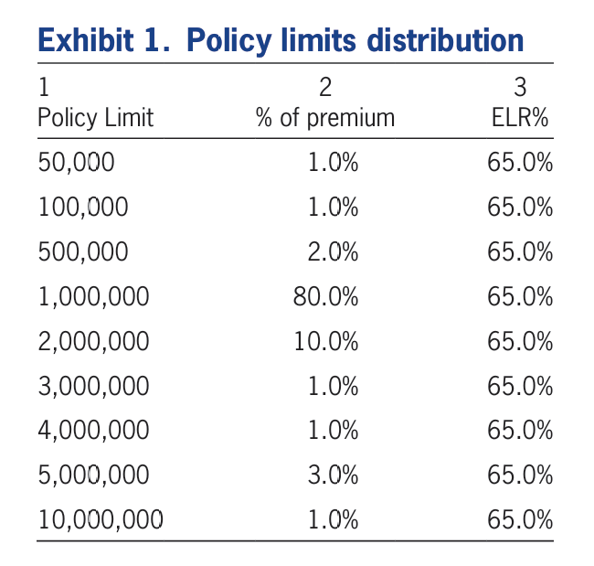
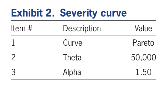
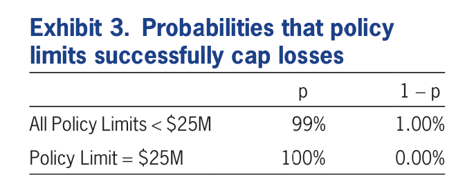
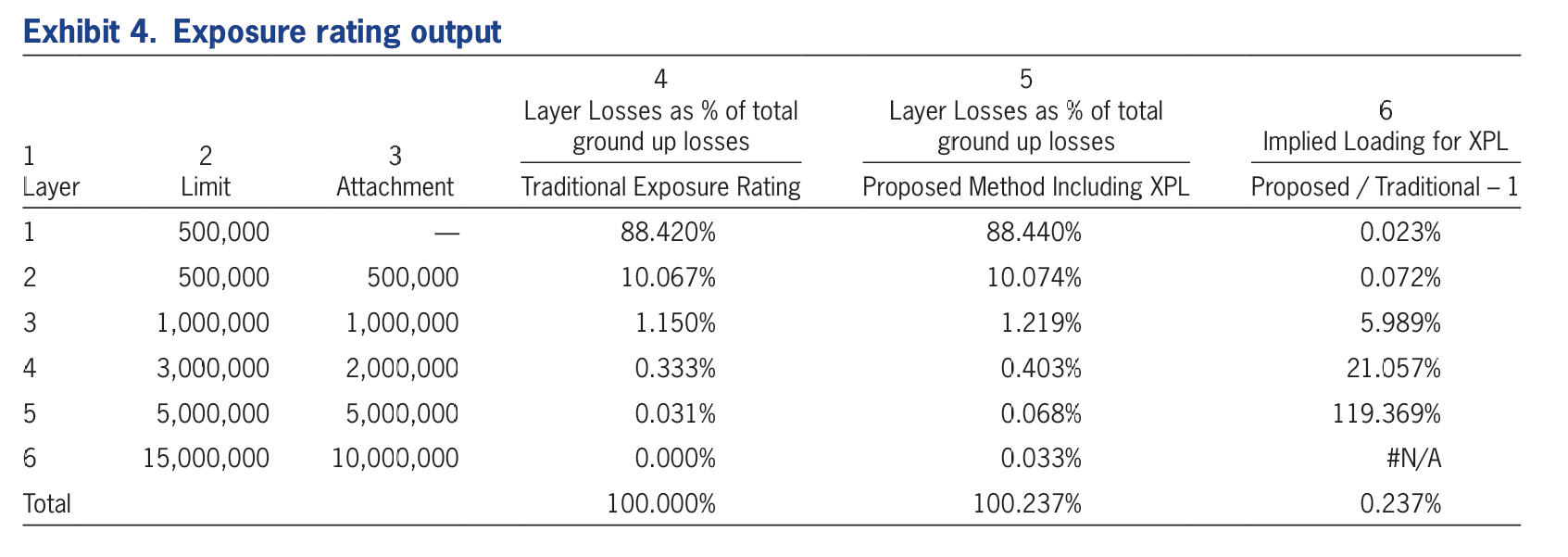
The reproduction target is Exhibit 4, Figure 2, the six-layer exposure rating. Its inputs are the three short exhibits in Figure 1: a nine-point policy limits profile with premium weights (Figure 1 (a)), a Pareto severity with \(\theta = 50{,}000\) and \(\alpha = 1.50\) (Figure 1 (b)), and \(p = 99\%\) for every policy limit below $25M (Figure 1 (c)).
The layer exposure factor, the paper’s equation (3.12), is
with \(T\) and \(B\) the top and bottom of the reinsurance layer. Traditional exposure rating is the same expression at \(p = 1\).
Two model choices in those three exhibits are not spelled out and have to be inferred.
“Pareto, theta 50,000, alpha 1.50” means the two parameter Pareto, \(S(x) = (\theta/(\theta+x))^\alpha\), the form in Clark’s reinsurance study note that the paper cites, not the single parameter Pareto supported on \([\theta, \infty)\). In DecL this is lomax.
Exhibit 3’s row “Policy Limit = $25M, p = 100%” is a global cap, not a row of the limits profile. No policy in Exhibit 1 has a $25M limit. The row is saying that the XPL branch is itself capped at $25M, which is what makes the six layers a complete tower: they run 0 to $500k, $500k to $1M, $1M to $2M, $2M to $5M, $5M to $10M, $10M to $25M, and the total of Figure 2 is the whole tower.
(a) Exhibit 1, the policy limits distribution.
(b) Exhibit 2, the severity curve.
(c) Exhibit 3, the probabilities that policy limits cap losses.
Figure 1: Bodoff (2017), Exhibits 1 to 3, the three inputs to the exposure rating.
Every quantity in Exhibit 4 is a limited expected value of the severity, and a limited expected value is what a single fixed claim in the layer a xs 0 costs. That is one build call.
def lev(a, log2=20):"""E[X and a] as the expected loss of one fixed claim in the layer a xs 0."""return build(f'agg B 1 claim {a} xs 0 sev {THETA} * lomax {ALPHA} fixed', log2=log2, bs=a /2** (log2 -2), normalize=False).est_mdef closed_form(a):"""theta/(alpha-1) [1 - (theta/(theta+a))^(alpha-1)]."""return THETA / (ALPHA -1) * (1- (THETA / (THETA + a)) ** (ALPHA -1))pts =sorted(set(LIMITS) | {CAP} | {t + y for y, t in LAYERS}| {t for y, t in LAYERS} - {0})LEV = {a: lev(a) for a in pts}chk = pd.DataFrame({'a': pts, 'aggregate': [LEV[a] for a in pts],'closed form': [closed_form(a) for a in pts]})chk['relative error'] = (chk['aggregate'] / chk['closed form'] -1).abs()GT(chk)
Table 1: Limited expected values of the Pareto severity at every breakpoint the exhibit needs, against the closed form.
a
aggregate
closed form
relative error
50,000
29,289
29,289
1.28e-12
100,000
42,265
42,265
4.03e-12
500,000
69,849
69,849
6.49e-11
1,000,000
78,178
78,178
2.33e-10
2,000,000
84,383
84,383
8.62e-10
3,000,000
87,196
87,196
1.88e-09
4,000,000
88,889
88,889
3.27e-09
5,000,000
90,050
90,050
5.05e-09
10,000,000
92,947
92,947
1.96e-08
25,000,000
95,532
95,532
1.19e-07
In Table 1, aggregate agrees with the closed form to within 1.2 parts in ten million at every limit, so the exposure rating rests on the severity and the arithmetic, not on the grid.
Table 2: Exhibit 4 rebuilt, the six layer tower at \(p = 1\) and at \(p = 99%\) with the implied XPL loading.
Layer
traditional %
proposed %
XPL loading %
$500k xs 0k
88.420
88.440
0.023
$500k xs 500k
10.067
10.074
0.072
$1,000k xs 1,000k
1.150
1.219
5.989
$3,000k xs 2,000k
0.333
0.403
21.057
$5,000k xs 5,000k
0.031
0.068
119.369
$15,000k xs 10,000k
0.000
0.033
—
Total
100.000
100.237
0.237
Table 3 transcribes what Exhibit 4 prints, for comparison with Table 2.
Table 3: Bodoff (2017), Exhibit 4 as printed.
Layer
Traditional
Proposed
Loading
$500k xs 0
88.420%
88.440%
0.023%
$500k xs $500k
10.067%
10.074%
0.072%
$1M xs $1M
1.150%
1.219%
5.989%
$3M xs $2M
0.333%
0.403%
21.057%
$5M xs $5M
0.031%
0.068%
119.369%
$15M xs $10M
0.000%
0.033%
n/a
Total
100.000%
100.237%
0.237%
Every cell matches to the precision printed, including the 119.369% loading on $5M xs $5M and the 0.237% total. The two inferred model choices are therefore confirmed: had either the Pareto form or the $25M cap been read wrongly, the top two layers would have missed by far more than a rounding.
4 Comments
4.1 The result the paper is selling
Bodoff’s point is not the total, which is a modest 0.237% load on the whole tower. It is the shape of column 6, isolated in Table 4.
sh = ex4.drop('Total')[['attachment', 'traditional %', 'proposed %','XPL loading %']].copy()sh['share of gross loss'] = sh['proposed %'] / ex4.loc['Total', 'proposed %']GT(sh.set_index('attachment'))
Table 4: The XPL loading by attachment, beside each layer’s share of gross loss.
attachment
traditional %
proposed %
XPL loading %
share of gross loss
0
88.42
88.44
0.02
0.88231
500,000
10.07
10.07
0.07
0.10050
1,000,000
1.15
1.22
5.99
0.01216
2,000,000
0.33
0.40
21.06
0.00402
5,000,000
0.03
0.07
119.37
0.00068
10,000,000
0.00
0.03
—
0.00033
In Table 4 one parameter, a single flat \(p = 99\%\) applied to every policy, produces XPL loadings that run from 2 basis points on the working layer to 119% on $5M xs $5M and to an infinite relative load on $15M xs $10M, where traditional exposure rating returns exactly zero because no policy in the profile has a limit above $10M. That last column is the practical payoff: a layer that traditional exposure rating prices at zero is not in fact free, and the method gives a number for it rather than a shrug.
The loadings also depend on the limits profile and not only on \(p\), which is easy to miss. The 80% concentration at the $1M limit is what drives the loading pattern; a book written mostly at $5M limits would get a quite different column 6 from the same \(p\).
4.2 Where this sits for aggregate
This is a severity and layer exercise, not a compound distribution exercise. There is no frequency in the paper at all: Exhibit 4 is expressed in percentages of ground up loss, and the expected loss ratio of 65% in Exhibit 1 cancels out of every ratio. aggregate is doing one job here, computing \(\mathsf E[X \wedge a]\) for a heavy Pareto, and doing it to eight figures.
That said, the paper’s section 3.1.1 sketches exactly the collective risk model aggregate is for: simulate a loss, simulate the policy limit attached to it, then simulate \(Z\) and cap or do not cap. In DecL that whole construction is a mixed severity, since a Bernoulli mixture of a limited and an unlimited curve is just a two point severity mixture, and the surrounding frequency comes free. Bodoff’s parsimony argument, that XPL “is not a completely new entity” but the same size of loss distribution read without a cap, is exactly what makes it expressible.
4.3 A caveat on the severity
Bodoff2017.Pareto is one of the curves already transcribed into actuarial-severity-curves.agg. With \(\alpha = 1.5\) it has infinite variance, so it raises InfiniteVarianceError if built unlimited. Every use here is inside a layer, which bounds it. The mean is finite, \(\theta/(\alpha-1) = 100{,}000\), and the $25M cap in Exhibit 3 brings even the XPL branch down to 95,532.
Programs in the aggregate Loss Lab
Each program below opens in the aggregate Loss Lab, which builds it with nothing to install. The names are those in reproductions.agg, where every program is renamed by its paper’s citation key.
Bodoff2017.B: Exhibit 4's Pareto severity under a policy limit.
Bodoff2017.B.v2: Exhibit 4's Pareto severity under a policy limit.
4 Comments
4.1 The result the paper is selling
Bodoff’s point is not the total, which is a modest 0.237% load on the whole tower. It is the shape of column 6, isolated in Table 4.
In Table 4 one parameter, a single flat \(p = 99\%\) applied to every policy, produces XPL loadings that run from 2 basis points on the working layer to 119% on $5M xs $5M and to an infinite relative load on $15M xs $10M, where traditional exposure rating returns exactly zero because no policy in the profile has a limit above $10M. That last column is the practical payoff: a layer that traditional exposure rating prices at zero is not in fact free, and the method gives a number for it rather than a shrug.
The loadings also depend on the limits profile and not only on \(p\), which is easy to miss. The 80% concentration at the $1M limit is what drives the loading pattern; a book written mostly at $5M limits would get a quite different column 6 from the same \(p\).
4.2 Where this sits for
aggregateThis is a severity and layer exercise, not a compound distribution exercise. There is no frequency in the paper at all: Exhibit 4 is expressed in percentages of ground up loss, and the expected loss ratio of 65% in Exhibit 1 cancels out of every ratio.
aggregateis doing one job here, computing \(\mathsf E[X \wedge a]\) for a heavy Pareto, and doing it to eight figures.That said, the paper’s section 3.1.1 sketches exactly the collective risk model
aggregateis for: simulate a loss, simulate the policy limit attached to it, then simulate \(Z\) and cap or do not cap. In DecL that whole construction is a mixed severity, since a Bernoulli mixture of a limited and an unlimited curve is just a two point severity mixture, and the surrounding frequency comes free. Bodoff’s parsimony argument, that XPL “is not a completely new entity” but the same size of loss distribution read without a cap, is exactly what makes it expressible.4.3 A caveat on the severity
Bodoff2017.Paretois one of the curves already transcribed intoactuarial-severity-curves.agg. With \(\alpha = 1.5\) it has infinite variance, so it raisesInfiniteVarianceErrorif built unlimited. Every use here is inside a layer, which bounds it. The mean is finite, \(\theta/(\alpha-1) = 100{,}000\), and the $25M cap in Exhibit 3 brings even the XPL branch down to 95,532.