Denuit et al. on comonotonic allocations

Reproducing Denuit, Dhaene, Ghossoub and Robert (2025)

Author

Stephen J. Mildenhall

Published

2026-10-22 19:55 commit b5ca906+

1 Context and problem

A pool of \(n\) agents brings losses \(X_1, \dots, X_n\) and shares the total \(S = X_1 + \dots + X_n\). The conditional mean risk sharing rule, which Denuit (2020) and a line of papers after it develop as the natural rule for peer to peer insurance, gives agent \(i\) the share

\[\kappa_i(s) = \mathsf E[X_i \mid S = s].\]

It is fair in the obvious sense, since the shares add up to \(s\) and each has the right expectation, and it needs no risk measure or utility function to state.

It has a defect. An allocation is comonotonic when every share is a non-decreasing function of the pool total. Comonotonicity is the no-sabotage condition: if my share can fall when the pool’s loss rises, I have an interest in a larger total, and the interests of the participants are no longer aligned. Two results are folklore in the risk sharing literature: any feasible allocation is dominated in convex order by a comonotonic one, and an allocation is Pareto optimal for the convex order exactly when it is comonotonic. The conditional mean rule is not always comonotonic, so it is not always Pareto optimal.

Denuit et al. (2025) is about closing the gap constructively. Several proofs of the two folkloric results exist, but as the paper observes, none is “explicit enough to allow for an easy algorithmic implementation in practice”. Using majorization and an extension of a result of Lorentz and Shimogaki, the paper gives an algorithm that takes any allocation and returns a comonotonic one that improves every agent in convex order while preserving every agent’s expectation.

This is a good reproduction target for a reason that has nothing to do with insurance pricing. The object the paper is about, \(\kappa_i\), is not a special quantity here: it is the exeqa_ column of a portfolio’s density_df, the conditional expectation that aggregate already computes for capital allocation. And the paper’s algorithm ships in the library as Portfolio.make_comonotonic_allocations, so the reproduction exercises the implementation against the paper that specified it.

2 Paper solution and gold standard

Section 3.2 gives a fully specified three agent example. Agents 1 and 2 carry independent truncated exponentials on \([0, M]\) with density \(f(x) = \beta e^{-\beta x} / (1 - e^{-\beta M})\). Agent 3 carries, on \([0, N]\), a truncated equal mixture of an exponential with parameter \(\beta\) and a gamma with shape \(\alpha\) and the same \(\beta\), with density

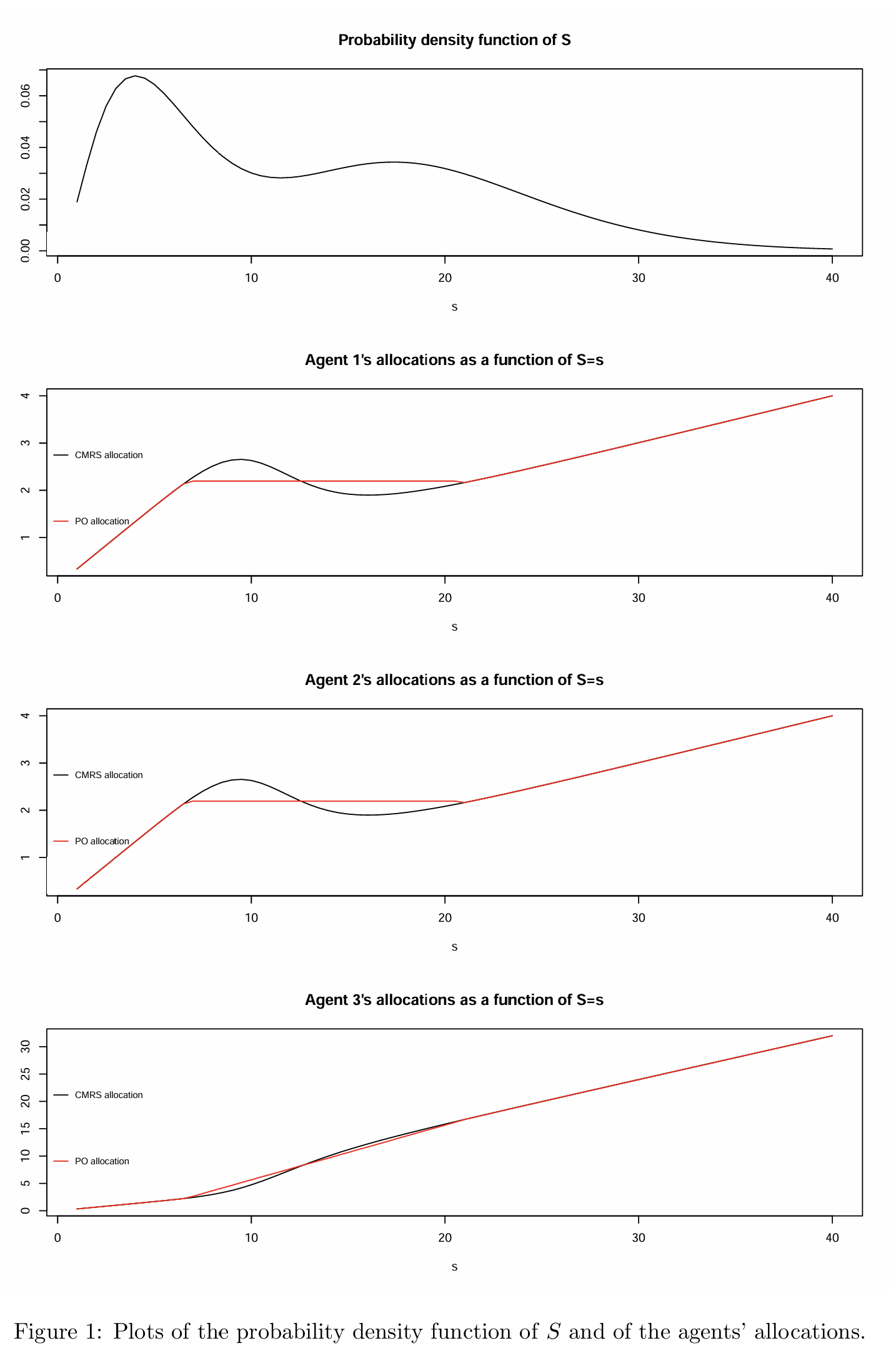
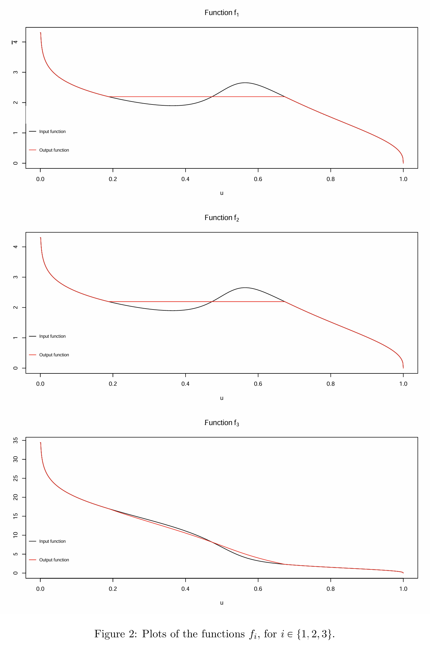
\[g(x) = \frac{\left(\beta + \beta^{\alpha} x^{\alpha - 1} / \Gamma(\alpha)\right) e^{-\beta x}}{\int_0^N \left(\beta + \beta^{\alpha} t^{\alpha - 1} / \Gamma(\alpha)\right) e^{-\beta t}\,\mathrm dt}.\]

The numerical illustration takes \(\beta = 1/2\), \(M = 10\), \(\alpha = 8\) and \(N = 30\). Figure 1, Figure 1, plots the density of \(S\) and, for each agent, the conditional mean allocation against the Pareto optimal improvement. Figure 2, Figure 3, plots the algorithm’s internal functions \(f_i\) on \([0, 1]\).

The paper prints no table, so the gold standard is the shape of Figure 1 plus two statements in the text: that the allocation functions of agents 1 and 2 are not increasing in \(s\), and that the algorithm replaces the initial functions by constants on an interval containing the decreasing parts while preserving expectations.

Note what the printed \(g\) says about the mixture weights. It is the sum of the two untruncated densities renormalized over \([0, N]\), so the equal weights cancel in the ratio. That is not the same as an equal mixture of the two individually truncated densities, because the two truncation constants differ: the exponential has essentially all its mass below 30 while the gamma with mean 16 does not. Written as a mixture of truncated components, the weights are proportional to \(\tfrac12 F_{\text{component}}(N)\), which Table 1 evaluates.

%xmode minimal
import numpy as np
import pandas as pd
import scipy.stats as ss
import matplotlib.pyplot as plt
from aggregate.constants import FIG_W, FIG_H
from bookstyle import GT, build, show

BETA, M, ALPHA, N = 0.5, 10.0, 8.0, 30.0
SCALE = 1 / BETA
EX, GM = ss.gamma(1, scale=SCALE), ss.gamma(ALPHA, scale=SCALE)
W = np.array([0.5 * EX.cdf(N), 0.5 * GM.cdf(N)])
W = W / W.sum()
GT(pd.DataFrame([
    {'quantity': 'F_exponential(N)', 'value': EX.cdf(N)},
    {'quantity': 'F_gamma(N)', 'value': GM.cdf(N)},
    {'quantity': 'weight on the truncated exponential', 'value': W[0]},
    {'quantity': 'weight on the truncated gamma', 'value': W[1]},
]).set_index('quantity'), float_format=10)

Exception reporting mode: Minimal

Table 1: The two truncation constants and the mixture weights they imply for agent 3.

quantity	value
F_exponential(N)	0.9999996941
F_gamma(N)	0.9819978069
weight on the truncated exponential	0.5045413496
weight on the truncated gamma	0.4954586504

3 The `aggregate` reproduction

A truncated distribution is a splice, and a mixture is a multi-component severity, so each agent is one agg and the pool is one port. Each agent takes a fixed frequency of one claim, so the aggregate is the risk.

# The trailer belongs on the `port` header line. Written after the last unit it
# binds to that unit, because the portfolio's trailer slot closes before the
# units are read, and the pool would then be auto-sized.
POOL = (f'port Denuit.Pool hints{{log2=16; bs=0.002; normalize=False; padding=1}}\n'
        f'    agg Agent1 1 claim sev {SCALE:g} * expon splice [0] [{M:g}] fixed\n'
        f'    agg Agent2 1 claim sev {SCALE:g} * expon splice [0] [{M:g}] fixed\n'
        f'    agg Agent3 1 claim sev {SCALE:g} * gamma [1 {ALPHA:g}] '
        f'wts [{W[0]:.12g} {W[1]:.12g}] splice [0 0] [{N:g} {N:g}] fixed\n')
pool = build(POOL)
show(pool)

port Denuit.Pool
  hints{log2=16; bs=0.002; normalize=False; padding=1}
  agg Agent1
    1 claim
    sev 2 * expon splice [0 10]
    fixed
  agg Agent2
    1 claim
    sev 2 * expon splice [0 10]
    fixed
  agg Agent3
    1 claim
    sev 2 * gamma [1 8] wts [0.504541349633 0.495458650367] splice [0 0] [30 30]
    fixed

The transcription needs an acceptance test, and the marginal means supply one: they are one dimensional integrals against the paper’s own densities, computable by quadrature without any of the machinery under test, as Table 2 does.

m12 = EX.expect(lambda x: x, lb=0, ub=M) / EX.cdf(M)
m3 = ((0.5 * EX.expect(lambda x: x, lb=0, ub=N)
       + 0.5 * GM.expect(lambda x: x, lb=0, ub=N))
      / (0.5 * EX.cdf(N) + 0.5 * GM.cdf(N)))
GT(pd.DataFrame([
    {'quantity': 'E[X_1] = E[X_2]', 'quadrature': m12,
     'aggregate': pool.agg_list[0].est_m},
    {'quantity': 'E[X_3]', 'quadrature': m3, 'aggregate': pool.agg_list[2].est_m},
    {'quantity': 'E[S]', 'quadrature': 2 * m12 + m3, 'aggregate': pool.est_m},
]).set_index('quantity'), float_format=8)

Table 2: The marginal means and the pool mean, by quadrature against the paper’s densities and from the build.

quantity	quadrature	aggregate
E[X_1] = E[X_2]	1.93216345	1.93216337
E[X_3]	8.77944917	8.77944913
E[S]	12.64377607	12.64377586

Two structural invariants follow from the specification rather than from the paper, and both are exact statements that a wrong build would break. Agents 1 and 2 are identically distributed, so \(\kappa_1 \equiv \kappa_2\) everywhere. And any allocation of \(S\) adds up, so \(\sum_i \kappa_i(s) = s\) at every \(s\). Table 3 tests both.

kap = [pool.density_df[f'exeqa_Agent{i}'] for i in (1, 2, 3)]
sl = (pool.density_df.index >= 0.5) & (pool.density_df.index <= 45)
tot = sum(k[sl] for k in kap)
GT(pd.DataFrame([
    {'invariant': 'max |kappa_1 - kappa_2| over s in [0.5, 45]',
     'value': float(np.abs(kap[0][sl] - kap[1][sl]).max())},
    {'invariant': 'max |sum of kappa_i minus s|',
     'value': float(np.abs(tot - tot.index).max())},
]).set_index('invariant'), formatters={'value': '{x:.2e}'})

Table 3: Symmetry of agents 1 and 2, and adding up, at numerical precision.

invariant	value
max \|kappa_1 - kappa_2\| over s in [0.5, 45]	0.00e+00
max \|sum of kappa_i minus s\|	1.58e-10

Now the allocation itself, and the paper’s claim about it, in Table 4.

GT(pd.DataFrame([{'s': s, 'kappa_1 = kappa_2': float(kap[0].loc[s]),
                  'kappa_3': float(kap[2].loc[s]),
                  'sum': float(sum(k.loc[s] for k in kap))}
                 for s in (5, 10, 15, 20, 25, 30, 35, 40, 45)]).set_index('s'),
   float_format=5)

Table 4: The conditional mean allocation at nine values of the pool total, with the shares totalled back to \(s\).

s	kappa_1 = kappa_2	kappa_3	sum
5	1.66276	1.67449	5.00000
10	2.63104	4.73793	10.00000
15	1.78877	11.42245	15.00000
20	2.01153	15.97694	20.00000
25	2.42093	20.15814	25.00000
30	2.78147	24.43705	30.00000
35	4.19309	26.61381	35.00000
40	6.07707	27.84586	40.00000
45	8.17604	28.64793	45.00000

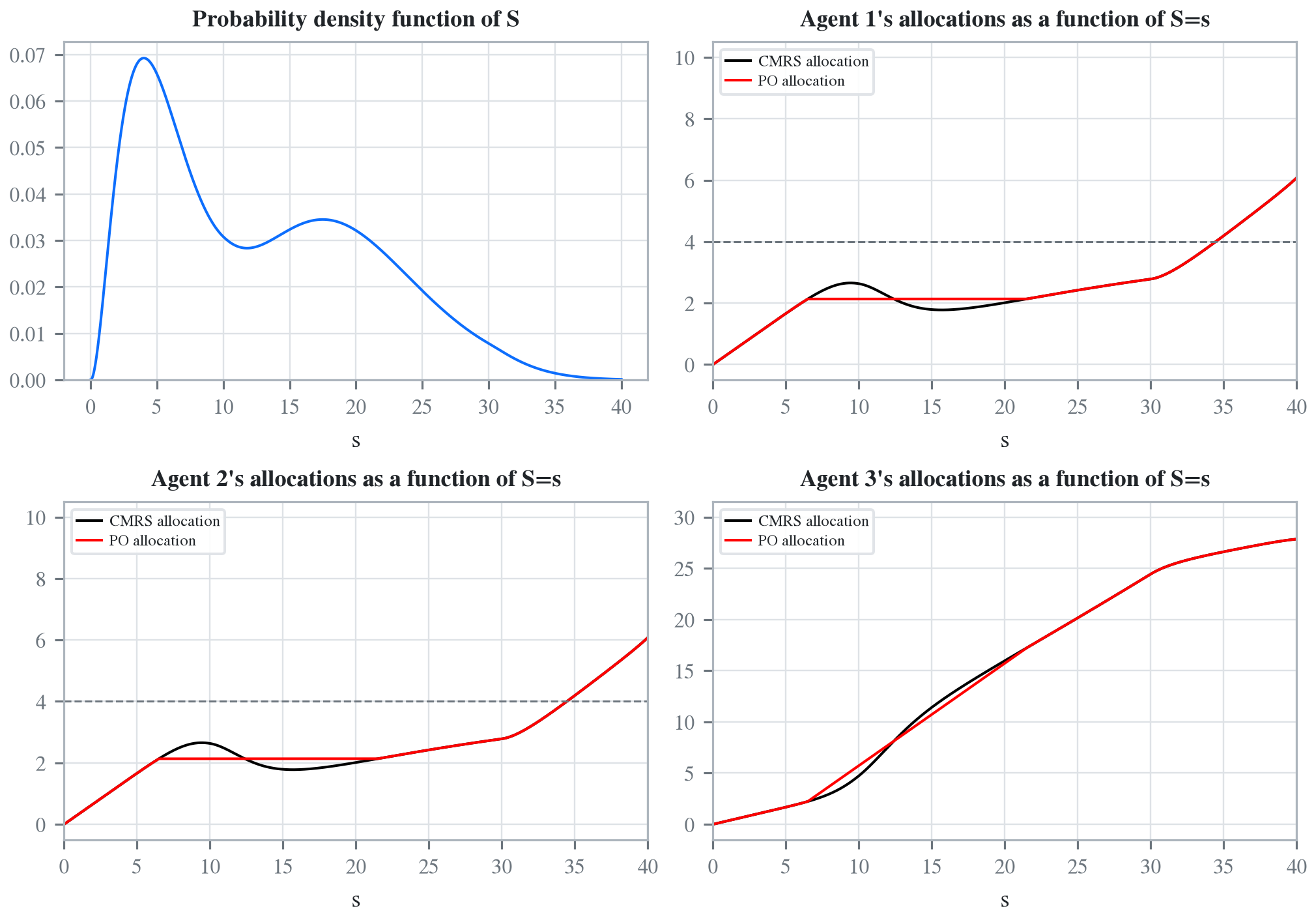
The paper’s claim reproduces in Table 4. Agents 1 and 2 rise to 2.631 at \(s = 10\), fall to 1.789 by \(s = 15\), and rise again thereafter, so the conditional mean allocation is not comonotonic and therefore not Pareto optimal. Agent 3 is increasing throughout, and Table 5 measures the dip.

rows = []
for i in (1, 2, 3):
    k = kap[i - 1][sl].to_numpy()
    d = np.diff(k)
    rows.append({'agent': i, 'decreasing steps %': 100 * float((d < 0).mean()),
                 'local max before the dip': float(k[:len(k) // 3].max()),
                 'value at the bottom of the dip': float(k[k[:len(k) // 3].argmax():].min())})
GT(pd.DataFrame(rows).set_index('agent'), float_format=4)

Table 5: How much of each agent’s allocation is decreasing, and the size of the dip.

agent	decreasing steps %	local max before the dip	value at the bottom of the dip
1	14.0584	2.6546	1.7772
2	14.0584	2.6546	1.7772
3	0.0000	11.7718	11.7718

3.1 Figure 1

Figure 1: Denuit, Dhaene, Ghossoub and Robert (2025), Figure 1.

comon = pool.make_comonotonic_allocations(max_loss=50)
fig, axs = plt.subplots(2, 2, figsize=(2 * FIG_W, 2 * FIG_H), layout='constrained')
d = pool.density_df.loc[:40]
axs[0, 0].plot(d.index, d.p_total / pool.bs, lw=1, c='C0')
axs[0, 0].set(title='Probability density function of S', xlabel='s', ylim=(0, None))
for i, ax in zip((1, 2, 3), axs.flat[1:]):
    ax.plot(comon.index, comon[f'exeqa_Agent{i}'], lw=1, c='k', label='CMRS allocation')
    ax.plot(comon.index, comon[f'exeqa_Agent{i}_t'], lw=1, c='r', label='PO allocation')
    ax.set(title=f"Agent {i}'s allocations as a function of S=s", xlabel='s', xlim=(0, 40))
    if i < 3:
        ax.axhline(4, ls='--', lw=0.75, c='C7')
    ax.legend(loc='upper left', fontsize=6)

Figure 2: Reproducing Figure 1. Black is the conditional mean allocation, red the Pareto optimal improvement. The dashed line on the agent 1 and 2 panels marks the top tick of the published axis.

Figure 2 is the reproduction of the picture. The algorithm’s three defining properties are checkable too, and they matter more than the picture: the output is non-decreasing, it preserves every expectation, and it still adds up. Table 6 and Table 7 take those in turn.

Figure 3: Denuit, Dhaene, Ghossoub and Robert (2025), Figure 2.

p = comon['p_total'].to_numpy()
rows = []
for i in (1, 2, 3):
    t = comon[f'exeqa_Agent{i}_t'].to_numpy()
    rows.append({
        'agent': i,
        'smallest step in the PO allocation': float(np.diff(t).min()),
        'E[CMRS share]': float((comon[f'exeqa_Agent{i}'].to_numpy() * p).sum()),
        'E[PO share]': float((t * p).sum())})
po_total = sum(comon[f'exeqa_Agent{i}_t'] for i in (1, 2, 3))
GT(pd.DataFrame(rows).set_index('agent'),
   formatters={'smallest step in the PO allocation': '{x:.2e}',
               'E[CMRS share]': 8, 'E[PO share]': 8})

Table 6: The Pareto optimal allocation is non-decreasing and preserves each agent’s expectation.

agent	smallest step in the PO allocation	E[CMRS share]	E[PO share]
1	0.00e+00	1.93216337	1.93216337
2	0.00e+00	1.93216337	1.93216337
3	0.00e+00	8.77944913	8.77944913

GT(pd.DataFrame([{'max |sum of PO shares minus s|':
                      float(np.abs(po_total - po_total.index).max()),
                  'bucket size': pool.bs}]),
   formatters={'max |sum of PO shares minus s|': '{x:.2e}', 'bucket size': '{x:g}'})

Table 7: The Pareto optimal shares still sum to \(s\), within a single bucket.

max \|sum of PO shares minus s\|	bucket size
3.03e-03	0.002

In Table 6 every PO share is non-decreasing to the last bucket and every expectation is preserved to about \(7\times10^{-12}\), and in Table 7 the shares still sum to \(s\) within a single bucket. The algorithm did what the theorem says.

4 Comments

4.1 The published Figure 1 cannot be right at its right hand edge

This takes no computation. Agent 3’s loss is capped at \(N = 30\). At \(s = 40\), adding up gives \(\kappa_1 + \kappa_2 = 40 - \kappa_3 \ge 10\), and agents 1 and 2 are identically distributed, so \(\kappa_1 = \kappa_2 \ge 5\). The published panels for agents 1 and 2 carry ticks at 1, 2, 3 and 4 over a horizontal range of \(s\) from 0 to 40. A curve that reaches at least 5 at the right hand edge cannot fit.

Table 8 says the same thing and locates the crossing: \(\kappa_1\) passes 4 at about \(s = 34\), reaching 4.193 at \(s = 35\) and 6.077 at \(s = 40\).

GT(pd.DataFrame([
    {'s': s, 'kappa_1 = kappa_2': float(kap[0].loc[s]),
     'kappa_3': float(kap[2].loc[s]),
     'above the published axis top of 4': bool(float(kap[0].loc[s]) > 4)}
    for s in (25, 30, 34, 35, 40)]).set_index('s'), float_format=4)

Table 8: Where the allocation for agents 1 and 2 leaves the published vertical axis, whose top tick is 4.

s	kappa_1 = kappa_2	kappa_3	above the published axis top of 4
25	2.4209	20.1581	False
30	2.7815	24.4371	False
34	3.8424	26.3152	False
35	4.1931	26.6138	True
40	6.0771	27.8459	True

One change to the model, and only one, brings the curve back inside the published box: dropping the \(N = 30\) truncation of agent 3, so that its gamma component runs unbounded. Then \(\kappa_3\) is free to exceed 30 and agents 1 and 2 stay low, as Table 9 shows.

alt = build(
    f'port Denuit.PoolAlt hints{{log2=16; bs=0.002; normalize=False; padding=1}}\n'
    f'    agg A1 1 claim sev {SCALE:g} * expon splice [0] [{M:g}] fixed\n'
    f'    agg A2 1 claim sev {SCALE:g} * expon splice [0] [{M:g}] fixed\n'
    f'    agg A3 1 claim sev {SCALE:g} * gamma [1 {ALPHA:g}] wts [0.5 0.5] fixed\n')
ka = alt.density_df['exeqa_A1']
GT(pd.DataFrame([
    {'s': s, 'agent 3 truncated at N = 30 (the paper text)': float(kap[0].loc[s]),
     'agent 3 not truncated': float(ka.loc[s])}
    for s in (20, 25, 30, 35, 40)]).set_index('s'), float_format=4)

Table 9: The allocation to agents 1 and 2 with and without the \([0, N]\) truncation on agent 3.

s	agent 3 truncated at N = 30 (the paper text)	agent 3 not truncated
20	2.0115	2.0115
25	2.4209	2.4209
30	2.7815	2.7815
35	4.1931	3.0760
40	6.0771	3.3132

So Figure 1 is consistent with a computation in which the \([0, N]\) truncation of agent 3 was specified in the text but not applied. That is a guess about a cause, and the paper’s own text is the authority on the model, so this page keeps the truncation.

Nothing in the paper’s results turns on it. The theorems are about any allocation, the algorithm is verified above against its three defining properties, and the feature of Figure 1 that the paper is actually pointing at, the non-monotone stretch in agents 1 and 2 between \(s = 10\) and \(s = 15\), is exactly where the paper says it is.

4.2 Which mixture, and a number worth reconciling

The reading of \(g\) matters slightly. Taking the printed density literally gives \(\mathsf E[X_3] = 8.779\) and \(\mathsf E[S] = 12.644\). Reading it instead as an equal mixture of the two individually truncated components gives \(\mathsf E[X_3] = 8.842\) and \(\mathsf E[S] = 12.706\), as Table 10 sets out.

alt2 = build(
    f'port Denuit.PoolB hints{{log2=16; bs=0.002; normalize=False; padding=1}}\n'
    f'    agg B1 1 claim sev {SCALE:g} * expon splice [0] [{M:g}] fixed\n'
    f'    agg B2 1 claim sev {SCALE:g} * expon splice [0] [{M:g}] fixed\n'
    f'    agg B3 1 claim sev {SCALE:g} * gamma [1 {ALPHA:g}] wts [0.5 0.5] '
    f'splice [0 0] [{N:g} {N:g}] fixed\n')
kb = alt2.density_df['exeqa_B1']
GT(pd.DataFrame([
    {'reading': 'printed density, renormalized over [0, N]',
     'E[X_3]': pool.agg_list[2].est_m, 'E[S]': pool.est_m,
     'kappa_1(15)': float(kap[0].loc[15]), 'kappa_1(40)': float(kap[0].loc[40])},
    {'reading': 'equal mixture of individually truncated components',
     'E[X_3]': alt2.agg_list[2].est_m, 'E[S]': alt2.est_m,
     'kappa_1(15)': float(kb.loc[15]), 'kappa_1(40)': float(kb.loc[40])},
]).set_index('reading'), float_format=5)

Table 10: The two readings of the printed density \(g\), and how far apart they leave the means and the allocation.

reading	E[X_3]	E[S]	kappa_1(15)	kappa_1(40)
printed density, renormalized over [0, N]	8.77945	12.64378	1.78877	6.07707
equal mixture of individually truncated components	8.84159	12.70592	1.78406	6.07707

The printed formula settles it, since the equal weights cancel in the normalization, and that is the reading used above. The distinction is worth recording because the second reading is the more natural thing to write in code, the two differ in the third digit of \(\mathsf E[S]\), and in Table 10 they are indistinguishable in the allocation above \(s = 20\).

4.3 What `aggregate` is doing here, and what it is not

There is no compound distribution in this paper. Every agent has one claim with certainty, so the aggregate is the severity, the frequency machinery is idle, and what is being exercised is the conditional expectation kernel and the grid it runs on. That is the same kernel behind natural allocation and the distortion pricing surface, which is why a risk sharing paper with no insurance contract in it is a useful test: it reads the allocation columns directly and checks them against constraints, rather than against another allocation.

The grid does need care. At bs = 0.002 over \(2^{16}\) buckets the pool reaches 131, comfortably past the support cap of \(10 + 10 + 30 = 50\), and in Table 3 the conditional expectations satisfy the adding up identity to \(10^{-13}\). A coarse grid degrades \(\kappa\) before it degrades the mean, so adding up is the invariant to watch.

Programs in the aggregate Loss Lab

Each program below opens in the aggregate Loss Lab, which builds it with nothing to install. The names are those in reproductions.agg, where every program is renamed by its paper’s citation key.

Denuit2025a.Denuit.Pool.v2: Section 3.2's three agent pool of truncated severities.
Denuit2025a.Denuit.PoolAlt: Section 3.2's three agent pool of truncated severities.
Denuit2025a.Denuit.PoolB: Section 3.2's three agent pool of truncated severities.

Denuit, M. M. (2020). Investing in your own and peers’ risks: the simple analytics of P2P insurance. European Actuarial Journal. https://doi.org/10.1007/s13385-020-00238-x

Denuit, M. M., Dhaene, J., Ghossoub, M., & Robert, C. Y. (2025). Comonotonicity and Pareto optimality, with application to collaborative insurance. Insurance: Mathematics and Economics, 120, 1–16. https://doi.org/10.1016/j.insmatheco.2024.11.001