Wang (2002) proposes the Wang transform as a single pricing framework covering financial and insurance risks. The transform distorts the survival function by
with \(\lambda\) a market price of risk. On a lognormal it reproduces Black-Scholes; on an insurance loss it produces the kind of loading actuaries recognize; and the paper’s argument is that this is not a coincidence but the point.
The weather derivative example is the interesting one for a reproduction, because it is the case where no parametric model is used at all. The underlying is Heating Degree Days for December at a weather station, and the only thing available is 22 years of history. There is no lognormal to transform, no fitted severity, and nothing to estimate beyond the empirical distribution itself. The transform is applied directly to 22 equally weighted observations.
That makes it a good test of a specific thing: whether aggregate can carry a purely empirical distribution through a distortion and price a derivative on it, with no parametric step anywhere.
2 Paper solution and gold standard
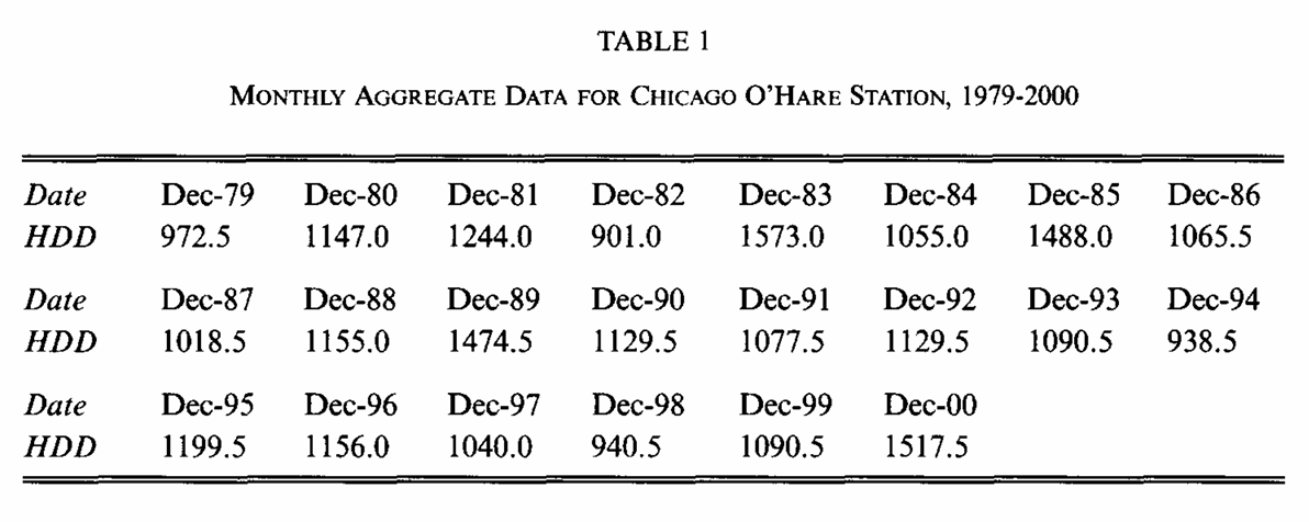
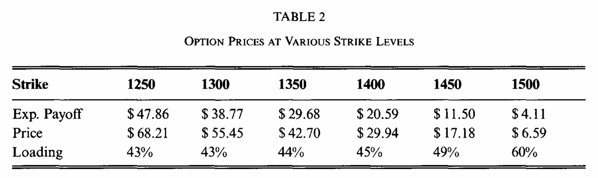
Table 1, Figure 1, lists the December HDD totals for 1979 to 2000, 22 observations. Table 2, Figure 2, prices call options on Dec-2001 HDDs at six strikes with \(\lambda = 0.25\), reporting the objective expected payoff, the transformed price, and the implied loading; Table 1 transcribes it.
The data transcription has an acceptance test that does not involve the transform at all. The objective expected payoff of a call struck at \(K\) is just \(\frac{1}{22}\sum_i (x_i - K)_+\), so if the 22 numbers are right, six of Table 2’s eighteen entries follow by arithmetic, as Table 2 confirms.
Table 2: The objective expected payoff at each strike straight from the 22 observations, against Table 2.
strike
empirical (x - K)+ mean
Table 2
difference
1,250
47.8636
47.86
0.0036
1,300
38.7727
38.77
0.0027
1,350
29.6818
29.68
0.0018
1,400
20.5909
20.59
0.0009
1,450
11.5000
11.50
0.0000
1,500
4.1136
4.11
0.0036
All six agree to within 0.004, which is the paper’s rounding to two decimals. The 22 observations are transcribed correctly, and the paper’s mean of 1,154.70 and standard deviation of 193.37 follow in Table 3.
Table 3: The two summary statistics the paper quotes for the December HDD record.
quantity
value
observations
22.0000
mean HDD
1,154.7045
standard deviation
193.3740
3 The aggregate reproduction
The empirical distribution goes in as a dsev, a discrete severity with one atom per observation, carried by a single certain claim so the aggregate is the empirical law.
bit = hdd.density_df.query('p_total > 0')[['p_total']]rows = []for k in PAPER.index:# push the atoms forward through the payoff map, then price the result payoff = bit.groupby(by=lambda x: np.maximum(0.0, x - k)).p_total.sum() p = d.price(payoff, kind='both') rows.append({'strike': k, 'expected payoff': p.el, 'price': p.ask,'loading %': 100* (p.ask / p.el -1), 'bid': p.bid})got = pd.DataFrame(rows).set_index('strike')GT(pd.concat({'paper': PAPER, 'aggregate': got[PAPER.columns]}, axis=1), float_format=2)
Table 4: Table 2 rebuilt, the expected payoff, transformed price and loading at all six strikes, beside the printed figures.
paper
aggregate
strike
expected payoff
price
loading %
expected payoff
price
loading %
1,250
47.86
68.21
43
47.86
68.21
42.50
1,300
38.77
55.45
43
38.77
55.45
43.02
1,350
29.68
42.70
44
29.68
42.70
43.84
1,400
20.59
29.94
45
20.59
29.94
45.40
1,450
11.50
17.18
49
11.50
17.18
49.42
1,500
4.11
6.59
60
4.11
6.59
60.08
rel = (got[PAPER.columns] / PAPER -1).abs()GT(pd.DataFrame([ {'column': c, 'worst absolute difference':float((got[c] - PAPER[c]).abs().max()),'worst relative difference': float(rel[c].max())}for c in PAPER.columns]).set_index('column'), formatters={'worst absolute difference': '{x:.4f}','worst relative difference': '{x:.2e}'})
Table 5: Worst absolute and relative difference from Table 2, column by column.
column
worst absolute difference
worst relative difference
expected payoff
0.0036
8.85e-04
price
0.0049
7.48e-04
loading %
0.4963
1.15e-02
In Table 4 and Table 5 all eighteen published entries reproduce to the precision printed. The expected payoffs agree to 0.004, within the paper’s two decimals. The six transformed prices, which depend on the whole machinery rather than on the data alone, agree to under half a cent: 68.21, 55.45, 42.70, 29.94, 17.18 and 6.59.
The loading row is printed as whole percentages and is the loosest of the three, since 42.50% at a strike of 1250 rounds to the paper’s 43% only just. That is a consequence of rounding a ratio of two rounded quantities rather than a disagreement: the price and the payoff it is formed from both match to four decimals.
4 Comments
4.1 The loading rises with the strike, and that is the interesting part
Table 6 puts the payoff probability beside the loading it earns.
GT(pd.DataFrame([ {'strike': k,'probability of payoff': float((h > k).mean()),'expected payoff': got.loc[k, 'expected payoff'],'price': got.loc[k, 'price'],'loading %': got.loc[k, 'loading %']}for k in PAPER.index]).set_index('strike'), formatters={'probability of payoff': 4, 'expected payoff': 3, 'price': 3,'loading %': 1})
Table 6: How often each strike pays, and the relative loading the transform puts on it.
strike
probability of payoff
expected payoff
price
loading %
1,250
0.1818
47.864
68.207
42.5
1,300
0.1818
38.773
55.451
43.0
1,350
0.1818
29.682
42.695
43.8
1,400
0.1818
20.591
29.939
45.4
1,450
0.1818
11.500
17.183
49.4
1,500
0.0909
4.114
6.585
60.1
In Table 6 the relative loading runs from 43% at a strike of 1250 to 60% at 1500, and the driver is visible in the first column: at 1250 the option pays in 9 of 22 years and at 1500 in 2 of 22. A distortion that reweights the survival function loads a thin, remote payoff more heavily than a frequent one, in relative terms, which is exactly the property Wang (2000) argues an insurance pricing operator should have. It is the same shape as the layer loadings in that paper, obtained here without a parametric severity anywhere in the calculation.
4.2 Twenty two observations is the whole model, and that is a real limitation
Nothing here smooths the data. The empirical distribution has 22 atoms, the distorted distribution has the same 22 atoms with reweighted probabilities, and the price is a weighted sum over them. That is faithful to the paper and it means the price at a strike above the largest observation is exactly zero, while the price just below it is determined by a single year, as Table 7 shows.
rows = []for k in (1500, 1520, 1550, 1573, 1600): payoff = bit.groupby(by=lambda x: np.maximum(0.0, x - k)).p_total.sum() p = d.price(payoff, kind='both') rows.append({'strike': k, 'years with a payoff': int((h > k).sum()),'expected payoff': p.el, 'price': p.ask})GT(pd.DataFrame(rows).set_index('strike'), formatters={'years with a payoff': 0, 'expected payoff': 4, 'price': 4})
Table 7: Prices at strikes reaching past the record, where the empirical distribution runs out of data.
strike
years with a payoff
expected payoff
price
1,500
2
4.1136
6.5851
1,520
1
2.4091
3.9668
1,550
1
1.0455
1.7215
1,573
0
0.0000
0.0000
1,600
0
0.0000
0.0000
In Table 7, past 1573, the highest December in the record, the option is free. Any real quote at those strikes needs a tail model, and the empirical route cannot supply one: this is the same limit Wang (2002) is working within, and the paper does not price above 1500. The reproduction inherits the limitation rather than papering over it, which is the right outcome, but it is worth stating that the method’s applicability stops where the data does.
4.3 Why this example is a useful test of the library rather than of the transform
The transform is a one line function and would be easy to check on a lognormal. What this example exercises is the plumbing around it: a discrete severity given as a list of 22 floats, a pushforward through a payoff map that collapses many atoms onto zero, and a distortion applied to the resulting distribution rather than to the original.
That pushforward is the step where a library is likely to be wrong, because the payoff map is not injective: every year below the strike maps to a payoff of exactly zero, so nine to twenty of the 22 atoms have to be merged and their probabilities added before the distortion is applied. Applying the distortion first and then mapping would give a different and wrong answer, since a distortion is not linear. The agreement to two decimals at all six strikes is evidence that the order is right.
Programs in the aggregate Loss Lab
Each program below opens in the aggregate Loss Lab, which builds it with nothing to install. The names are those in reproductions.agg, where every program is renamed by its paper’s citation key.
Wang2002.HDD: the 22 observed heating degree day totals as a discrete severity.
Wang2002.wang25: the Wang transform used to price the option.
Wang, S. S. (2000). A class of distorion operators for pricing financial and insurance risks. Journal of Risk and Insurance, 67(1), 15–36.
Wang, S. S. (2002). A Universal Framework for Pricing Financial and Insurance Risks. ASTIN Bulletin, 32(2), 213–234. https://doi.org/10.2143/AST.32.2.1027
4 Comments
4.1 The loading rises with the strike, and that is the interesting part
Table 6 puts the payoff probability beside the loading it earns.
In Table 6 the relative loading runs from 43% at a strike of 1250 to 60% at 1500, and the driver is visible in the first column: at 1250 the option pays in 9 of 22 years and at 1500 in 2 of 22. A distortion that reweights the survival function loads a thin, remote payoff more heavily than a frequent one, in relative terms, which is exactly the property Wang (2000) argues an insurance pricing operator should have. It is the same shape as the layer loadings in that paper, obtained here without a parametric severity anywhere in the calculation.
4.2 Twenty two observations is the whole model, and that is a real limitation
Nothing here smooths the data. The empirical distribution has 22 atoms, the distorted distribution has the same 22 atoms with reweighted probabilities, and the price is a weighted sum over them. That is faithful to the paper and it means the price at a strike above the largest observation is exactly zero, while the price just below it is determined by a single year, as Table 7 shows.
In Table 7, past 1573, the highest December in the record, the option is free. Any real quote at those strikes needs a tail model, and the empirical route cannot supply one: this is the same limit Wang (2002) is working within, and the paper does not price above 1500. The reproduction inherits the limitation rather than papering over it, which is the right outcome, but it is worth stating that the method’s applicability stops where the data does.
4.3 Why this example is a useful test of the library rather than of the transform
The transform is a one line function and would be easy to check on a lognormal. What this example exercises is the plumbing around it: a discrete severity given as a list of 22 floats, a pushforward through a payoff map that collapses many atoms onto zero, and a distortion applied to the resulting distribution rather than to the original.
That pushforward is the step where a library is likely to be wrong, because the payoff map is not injective: every year below the strike maps to a payoff of exactly zero, so nine to twenty of the 22 atoms have to be merged and their probabilities added before the distortion is applied. Applying the distortion first and then mapping would give a different and wrong answer, since a distortion is not linear. The agreement to two decimals at all six strikes is evidence that the order is right.