Denuit, Hieber and Robert on mortality credits

Reproducing Denuit, Hieber and Robert (2022), Example 4.5

Author

Stephen J. Mildenhall

Published

2026-10-22 19:55 commit b5ca906+

1 Context and problem

A survivor fund pays the accumulated savings of members who die to the members who survive. The payment each survivor receives is the mortality credit, and the question is how to split it fairly when members differ in both their savings $a_i$ and their death probability $q_i$.

Denuit et al. (2022) apply conditional mean risk sharing to this. Member $i$ contributes $X_i = a_i \mathbb 1\{\text{$i$ dies}\}$ to the pool, the pool total is $S_n = \sum_i X_i$, and the fair share is again $\mathsf E[X_i \mid S_n = s]$. The paper’s contribution for large pools is an asymptotic expansion of that conditional expectation, accurate to $O(n_j^{-3/2})$, so that a fund with thousands of members does not need an exact convolution to allocate credits.

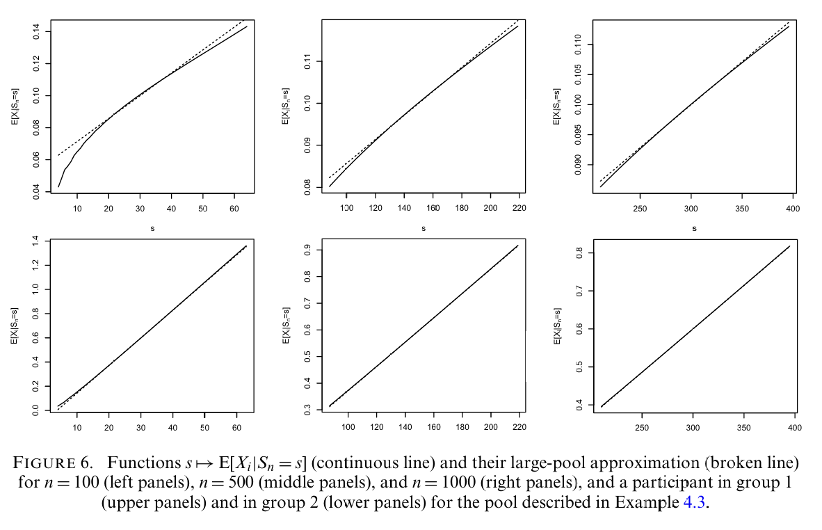
Example 4.5 illustrates the accuracy of that approximation, using the two group pool of Example 4.3, and its evidence is Figure 6, Figure 1.

2 Paper solution and gold standard

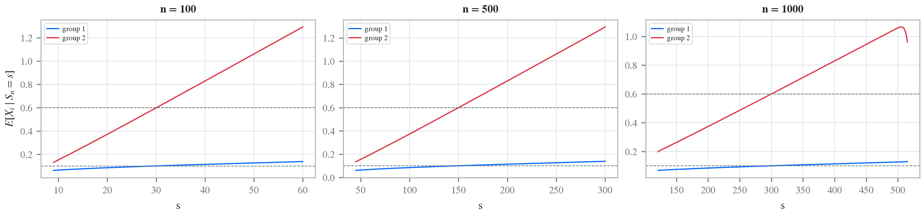
Example 4.3’s pool has two groups: group 1 is 60% of the pool with $a_i = 1$ and $q_i = 0.1$; group 2 is 40% with $a_i = 3$ and $q_i = 0.2$. Figure 6 plots $s \mapsto \mathsf E[X_i \mid S_n = s]$ for $n \in \{100, 500, 1000\}$.

The quantity plotted is per member, not per group, which is what fixes the axes. Its unconditional value is $a_i q_i$, so $0.1$ for group 1 and $0.6$ for group 2, and Figure 6’s first panel runs from 0.04 to 0.14 on the vertical axis over $s$ from 10 to 60. That is group 1 at $n = 100$, whose expected total is $\mathsf E[S_{100}] = 100(0.6 \cdot 1 \cdot 0.1 + 0.4 \cdot 3 \cdot 0.2) = 30$.

The paper prints no table, so the checks available are the axis ranges, the structural identities the allocation must satisfy whatever the picture looks like, and the convergence the example exists to demonstrate.

%xmode minimal
import numpy as np
import pandas as pd
import matplotlib.pyplot as plt
from aggregate.constants import FIG_W, FIG_H
from bookstyle import GT, build, show

W_LOW, W_HIGH = 0.6, 0.4
Q_LOW, Q_HIGH = 0.1, 0.2
A_LOW, A_HIGH = 1, 3
NS = (100, 500, 1000)

def fund(n):
    """Two groups of Bernoulli deaths. The count is binomial, the payout a_i."""
    return build(f'port Fund{n} '
                 f'agg Low  {W_LOW * n * Q_LOW} claims dsev [{A_LOW}] '
                 f'binomial {Q_LOW} '
                 f'agg High {W_HIGH * n * Q_HIGH} claims dsev [{A_HIGH}] '
                 f'binomial {Q_HIGH}', bs=1, log2=13)

funds = {n: fund(n) for n in NS}
show(funds[100])

Exception reporting mode: Minimal

port Fund100
  agg Low
    6 claims
    dsev [1]
    binomial 0.1
  agg High
    8 claims
    dsev [3]
    binomial 0.2

A member of group 1 dies with probability $q_{\text{low}}$ and then contributes $a_{\text{low}}$, so the group’s contribution is a binomial count of unit claims. In DecL the frequency clause is binomial q with an expected count of $w n q$, which is the group’s expected number of deaths. Table 1 checks the pool mean at all three sizes.

GT(pd.DataFrame([
    {'n': n, 'members in group 1': W_LOW * n, 'members in group 2': W_HIGH * n,
     'E[S] aggregate': funds[n].est_m,
     'E[S] exact': n * (W_LOW * A_LOW * Q_LOW + W_HIGH * A_HIGH * Q_HIGH)}
    for n in NS]).set_index('n'),
   formatters={'members in group 1': 0, 'members in group 2': 0,
               'E[S] aggregate': 6, 'E[S] exact': 6})

Table 1: Group sizes and the pool mean at each $n$, against the exact value.

n	members in group 1	members in group 2	E[S] aggregate	E[S] exact
100	60	40	30.000000	30.000000
500	300	200	150.000000	150.000000
1,000	600	400	300.000000	300.000000

3 The `aggregate` reproduction

By symmetry within a group, the per member conditional expectation is the group’s exeqa_ column divided by the number of members in that group. Table 2 samples it at three values of $s$ for each $n$.

def per_member(n):
    p = funds[n]
    d = p.density_df.query('p_total > 0')
    return pd.DataFrame(
        {'group 1': d['exeqa_Low'].to_numpy() / (W_LOW * n),
         'group 2': d['exeqa_High'].to_numpy() / (W_HIGH * n)},
        index=d.index)

pm = {n: per_member(n) for n in NS}
rows = []
for n, ss in zip(NS, ([20, 40, 60], [100, 150, 200], [200, 300, 400])):
    for s in ss:
        rows.append({'n': n, 's': s, 'group 1': pm[n].loc[s, 'group 1'],
                     'group 2': pm[n].loc[s, 'group 2'],
                     'sum times n': (pm[n].loc[s, 'group 1'] * W_LOW * n
                                     + pm[n].loc[s, 'group 2'] * W_HIGH * n)})
GT(pd.DataFrame(rows).set_index(['n', 's']), float_format=5)

Table 2: Per member conditional expectation for both groups at three values of $s$ per pool size, with the shares totalled back to $s$.

n	s	group 1	group 2	sum times n
100	20	0.08539	0.37192	20.00000
	40	0.11382	0.82927	40.00000
	60	0.13830	1.29255	60.00000
500	100	0.08453	0.37321	100.00000
	150	0.10013	0.59980	150.00000
	200	0.11355	0.82967	200.00000
1,000	200	0.08442	0.37338	200.00000
	300	0.10007	0.59990	300.00000
	400	0.11352	0.82972	400.00000

In Table 2, group 1 at $n = 100$ runs from 0.0854 at $s = 20$ to 0.1383 at $s = 60$, which sits inside Figure 1’s published vertical range of 0.04 to 0.14 over exactly that horizontal range. That is the identification of the panel, and it is the reason the per member normalization is the right reading of the figure.

3.1 Two exact identities

Table 3 tests both.

rows = []
for n in NS:
    p, d = funds[n], pm[n]
    nl, nh = W_LOW * n, W_HIGH * n
    tot = d['group 1'] * nl + d['group 2'] * nh
    es = round(n * (W_LOW * A_LOW * Q_LOW + W_HIGH * A_HIGH * Q_HIGH))
    rows.append({
        'n': n,
        'max |sum of shares minus s|': float(np.abs(tot - tot.index).max()),
        'group 1 share at s = E[S]': float(d.loc[es, 'group 1']),
        'a q for group 1': A_LOW * Q_LOW,
        'group 2 share at s = E[S]': float(d.loc[es, 'group 2']),
        'a q for group 2': A_HIGH * Q_HIGH})
GT(pd.DataFrame(rows).set_index('n'),
   formatters={'max |sum of shares minus s|': '{x:.1e}',
               'group 1 share at s = E[S]': 6, 'a q for group 1': 3,
               'group 2 share at s = E[S]': 6, 'a q for group 2': 3})

Table 3: Adding up, and the conditional expectation at the mean against the unconditional $a_i q_i$, at each pool size.

n	max \|sum of shares minus s\|	group 1 share at s = E[S]	a q for group 1	group 2 share at s = E[S]	a q for group 2
100	1.5e+00	0.100631	0.100	0.599053	0.600
500	6.3e+00	0.100131	0.100	0.599804	0.600
1,000	5.2e+01	0.100065	0.100	0.599902	0.600

In Table 3 the shares add up to $s$ exactly, at every $n$ and every $s$, which is the defining property of an allocation. And at $s = \mathsf E[S_n]$ the conditional expectation converges to the unconditional $a_i q_i$ as $n$ grows: group 1 goes 0.100631, 0.100131, 0.100065 against 0.1 as $n$ runs 100, 500, 1000, and group 2 goes 0.599053, 0.599804, 0.599902 against 0.6. The error falls by about a factor of two each time $n$ multiplies by roughly the same, and it is not exact at finite $n$, nor should it be, since the conditional expectation at the mean is not the mean of the conditional expectation.

3.2 Figure 6

Figure 1: Denuit, Hieber and Robert (2022), Figure 6.

fig, axs = plt.subplots(1, 3, figsize=(3 * FIG_W, FIG_H), layout='constrained')
for ax, n in zip(axs, NS):
    es = round(n * (W_LOW * A_LOW * Q_LOW + W_HIGH * A_HIGH * Q_HIGH))
    d = pm[n]
    sl = (d.index >= 0.3 * es) & (d.index <= 2.0 * es)
    ax.plot(d.index[sl], d.loc[sl, 'group 1'], lw=1, label='group 1')
    ax.plot(d.index[sl], d.loc[sl, 'group 2'], lw=1, label='group 2')
    ax.axhline(A_LOW * Q_LOW, ls='--', lw=0.6, c='C7')
    ax.axhline(A_HIGH * Q_HIGH, ls='--', lw=0.6, c='C7')
    ax.set(xlabel='s', title=f'n = {n}',
           ylabel='$E[X_i \\mid S_n = s]$' if n == 100 else '')
    ax.legend(fontsize=6)

Figure 2: Reproducing Figure 6. Per member conditional expectation for the two groups, at n = 100, 500 and 1000. Dashed lines are the unconditional a q.

Both curves in Figure 2 increase in $s$, so the allocation is comonotonic here and therefore Pareto optimal in the sense of Denuit et al. (2025), without needing that paper’s repair. That is worth noting because it is not automatic: the non-monotone case in Denuit et al. (2025) arose from a heavy tailed mixture, and a Bernoulli pool is about as far from that as a risk sharing model gets.

3.3 The convergence the example is about

The point of Example 4.5 is that the shape stabilizes as $n$ grows, which is what licenses the asymptotic approximation. Comparing the three panels at proportionally equal positions isolates that, in Table 4.

rows = []
for frac in (0.6, 0.8, 1.0, 1.3, 1.6):
    r = {'s / E[S]': frac}
    for n in NS:
        es = round(n * (W_LOW * A_LOW * Q_LOW + W_HIGH * A_HIGH * Q_HIGH))
        r[f'n = {n}'] = float(pm[n].loc[round(frac * es), 'group 1'])
    rows.append(r)
conv = pd.DataFrame(rows).set_index('s / E[S]')
conv['|500 - 1000|'] = (conv['n = 500'] - conv['n = 1000']).abs()
conv['|100 - 1000|'] = (conv['n = 100'] - conv['n = 1000']).abs()
GT(conv, formatters={'n = 100': 6, 'n = 500': 6, 'n = 1000': 6,
                     '|500 - 1000|': '{x:.2e}', '|100 - 1000|': '{x:.2e}'})

Table 4: Group 1’s per member share at fixed multiples of the mean, at each pool size, with the residual dependence on $n$.

s / E[S]	n = 100	n = 500	n = 1000	\|500 - 1000\|	\|100 - 1000\|
0.600	0.081898	0.080927	0.080801	1.25e-04	1.10e-03
0.800	0.091849	0.091164	0.091074	9.03e-05	7.75e-04
1.000	0.100631	0.100131	0.100065	6.53e-05	5.66e-04
1.300	0.112556	0.112267	0.112230	3.66e-05	3.25e-04
1.600	0.123715	0.123612	0.123600	1.27e-05	1.16e-04

In Table 4, at a fixed multiple of the mean the per member share is nearly independent of $n$, and the residual dependence shrinks by roughly the factor the paper’s $O(n_j^{-3/2})$ rate implies between $n = 500$ and $n = 1000$. So the curves in Figure 1 do lie on top of each other once the horizontal axis is scaled, which is the qualitative claim, and it is the reason an approximation depending only on the group’s aggregate moments can work.

4 Comments

4.1 An earlier treatment plotted a different quantity

The user guides version of this example builds the same pool but at $n \in \{10, 20, 50, 100\}$ rather than the paper’s $\{100, 500, 1000\}$, and plots the exeqa_ columns directly, which are group totals rather than per member shares. At $n = 100$ that is a factor of 60 and 40 away from the paper’s vertical axis.

Neither difference is an error in itself, since the group total is a perfectly good thing to look at and small pools are instructive. They do mean the earlier figure is not Figure 1, and the small $n$ end is where the paper’s approximation is least accurate, so the panels least like the published ones are the ones chosen.

4.2 Why a Bernoulli pool needs no discretization care

bs = 1 is exact here and no grid argument is needed anywhere on this page. Both payouts, 1 and 3, are integers, so the pool total lives on the integer lattice and the FFT convolution is exact up to floating point. That is visible in Table 3: the shares add to $s$ to $10^{-12}$ rather than to a bucket.

It also means the reproduction is testing the conditional expectation kernel with nothing else in the way. Where the Denuit et al. (2025) chapter had to argue about grid resolution before it could trust $\kappa$, this one does not, so the exact adding up at three pool sizes is direct evidence about the kernel rather than about the discretization around it.

4.3 What the fund actually pays

One thing worth making explicit, because the model is compact enough to obscure it: $\mathsf E[X_i \mid S_n = s]$ is what member $i$ contributes, so the mortality credit a survivor receives is funded by the difference between the pool’s realized total and the contributions of those who died. The allocation question the paper solves is the fair split of the contribution side, and the reason it is not trivial is that group 2 members bring three times the savings at twice the death probability, so a large $s$ is much more likely to have come from group 2 and the split has to reflect that. The curves above are exactly that reflection: at $s = 2\,\mathsf E[S]$ group 2’s per member share is well above its unconditional $0.6$ while group 1’s has barely moved off $0.1$.

Programs in the aggregate Loss Lab

Each program below opens in the aggregate Loss Lab, which builds it with nothing to install. The names are those in reproductions.agg, where every program is renamed by its paper’s citation key.

Denuit2022b.Fund100: Example 4.5's two group mortality pool at n = 100.
Denuit2022b.Fund500: Example 4.5's two group mortality pool at n = 500.

Denuit, M. M., Dhaene, J., Ghossoub, M., & Robert, C. Y. (2025). Comonotonicity and Pareto optimality, with application to collaborative insurance. Insurance: Mathematics and Economics, 120, 1–16. https://doi.org/10.1016/j.insmatheco.2024.11.001

Denuit, M. M., Hieber, P., & Robert, C. Y. (2022). Mortality Credits Within Large Survivor Funds. ASTIN Bulletin, 52(3), 813–834. https://doi.org/10.1017/asb.2022.13