Klugman, Panjer and Willmot on aggregate loss models
Klugman, Panjer and Willmot (2019), Loss Models: From Data to Decisions, fifth edition, Chapter 9
Author
Stephen J. Mildenhall
Published
2026-10-22 19:57 commit b7145b5+
Examples from the text Klugman et al. (2019), Loss Models: from data to decisions. The Loss models book is used as a text for several actuarial society exams and many college courses. KPW is shorthand for Loss Models.
1 Method of Moments Approximations, Examples 9.3 and 9.4
The observed mean (and standard deviation) of the number of claims and the individual losses over the past 10 months are 6.7 (2.3) and 179,247 (52,141), respectively. Determine the mean and standard deviation of aggregate claims per month.
from aggregate import qd, mv, MomentAggregator, round_bucketimport scipy.stats as ssimport pandas as pdimport numpy as npimport matplotlib.pyplot as pltmoms = MomentAggregator.agg_from_fs2(6.7, 2.3**2, 179247, 52141**2)moms
ex     1.200955e+06
var    1.881802e+11
sd     4.337974e+05
cv     3.612104e-01
dtype: float64
Using normal and lognormal distributions as approximating distributions for aggregate claims, calculate the probability that claims will exceed 140% of expected costs.
Under a group dental insurance plan covering employees and their families, the premium for each married employee is the same regardless of the number of family members. The insurance company has compiled statistics showing that the annual cost of dental care per person for the benefits provided by the plan has the distribution (given in units of 25) on the left.
Furthermore, the distribution of the number of persons per insurance certificate (i.e. per employee) receiving dental care in any year has the distribution on the right.
Determine the mean and standard deviation of total payments per employee.
Exercise 9.19. An insurance portfolio produces N = 0, 1, 3 claims with probabilities 0.5, 0.4, 0.1. Individual claim amounts are 1 or 10 with probability 0.9, 0.1. Individual claim amounts and N are mutually independent. Calculate the probability that the ratio of aggregate claims to expected claims will exceed 3.0.
Aggregate object: KPW.9.19. Frequency distribution empirical. Severity
dhistogram, [1, 10], bounded; atoms [1 10]. Updated with bucket size 1
and log2 = 5. Validation: not unreasonable.

      Mean     SD     CV   Skew P01 Median P99
X
Freq   0.7    0.9 1.2857 1.4486
Sev    1.9    2.7 1.4211 2.6667   1      1  10
Agg   1.33 2.8332 2.1302  3.414   0      0  12
mean        1.33
probability 0.0671
Exercise 9.23. An individual loss distribution is normal with mean = 100 and variance = 9. The distribution for the number of claims has outcomes 0, 1, 2, 3 with probabilities 0.5, 0.2, 0.2, 0.1. Determine the probability that aggregate claims exceed 100.
Aggregate object: KPW.9.23. Frequency distribution empirical. Severity
norm, [0, inf), super-exponential right tail. Updated with bucket size
1/32 and log2 = 16. Validation: fails sev skew.

      Mean     SD     CV    Skew    P01 Median    P99
X
Freq   0.9  1.044   1.16  0.7276
Sev    100      3   0.03       0 93.031    100 106.97
Agg     90 104.44 1.1605 0.72937      0      0 306.66

               p       F       S
loss
90.0  3.2132e-06 0.50009 0.49991
92.0  2.3742e-05 0.50078 0.49922
94.0  0.00011248 0.50461 0.49539
96.0  0.00034169 0.51841 0.48159
98.0  0.00066552 0.55083 0.44917
100.0 0.00083113 0.60042 0.39958
102.0 0.00066552 0.64983 0.35017
104.0 0.00034169 0.68193 0.31807
106.0 0.00011248 0.69551 0.30449
108.0 2.3742e-05 0.69925 0.30075
110.0 3.2132e-06 0.69992 0.30008
Exercise 9.24. An employer self-insures a life insurance program with the following two characteristics:
Given that a claim has occurred, the claim amount is 2,000 with probability 0.4 and 3,000 with probability 0.6.
The number of claims has outcomes 0, 1, 2, 3, 4 with probabilities 1/16, 1/4, 3/8, 1/4, 1/16.
The employer purchases aggregate stop-loss coverage that limits the employer’s annual claims cost to 5,000. The aggregate stop-loss coverage costs 1,472. Determine the employer’s expected annual cost of the program, including the cost of stop-loss coverage.
kpw_9_24 = build('agg KPW.9.24 dfreq [0:4] [1/16 1/4 3/8 1/4 1/16] ''dsev [2 3] [0.4 0.6] ''aggregate net of inf xs 5')qd(kpw_9_24)net = kpw_9_24.summary_df.loc['Agg', 'Mean']print(f'\ngross loss {kpw_9_24.actual_m:.5g}\nretained loss {net:.5g}\n'f'premium {net +1.472:.5g}')
Aggregate object: KPW.9.24. Frequency distribution empirical. Severity
dhistogram, [2, 3], bounded; atoms [2 3]. Updated with bucket size 1 and
log2 = 4. Validation: reinsurance; subject not unreasonable.

       Mean     SD      CV     Skew P01 Median P99
X
Freq      2      1     0.5        0
Sev     2.6 0.4899 0.18842 -0.40825   2      3   3
Agg  4.0275 1.4754 0.36633  -1.4019   0      5   5

gross loss    5.2
retained loss 4.0275
premium       5.4995
Working in thousands.
Exercise 9.31. Medical and dental claims are assumed to be independent with compound Poisson distributions as follows:
Medical claims 2 expected claims, amounts uniform (0, 1000)
Let X be the amount of a given claim under a policy that covers both medical and dental claims. Determine E[(X − 100)+], the expected cost (in excess of 100) of any given claim.
Aggregate object: KPW.9.31. Frequency distribution poisson. Mixed
severity with 2 components. Updated with bucket size 1/2 and log2 = 16.
Validation: reinsurance; subject not unreasonable.

      Mean     SD      CV    Skew P01 Median    P99
X
Freq     5 2.2361 0.44721 0.44721
Sev    177 258.59   1.461  1.4244   0     47    875
Agg    885 700.71 0.79177 0.95458   0  786.5 2952.5

                        EX  Est EX  Change EX      CV  Est CV  Change CV      Sk  Est Sk
stage view  component
occ   gross freq         5     NaN        NaN 0.44721     NaN        NaN 0.44721     NaN
            sev        260     260          0  1.0444  1.0444          0  1.3042  1.3042
            agg       1300    1300 -1.285e-12 0.64664 0.64664 -1.083e-11 0.85178 0.85178
      ceded freq         5       5          0 0.44721     NaN        NaN 0.44721     NaN
            sev        260     177   -0.31923  1.0444   1.461     0.3989  1.3042  1.4244
            agg       1300     885   -0.31923 0.64664 0.79177    0.22443 0.85178 0.95458
      net   freq         5       5          0 0.44721     NaN        NaN 0.44721     NaN
            sev        260      83   -0.68077  1.0444 0.35009   -0.66478  1.3042 -1.5092
            agg       1300     415   -0.68077 0.64664 0.47383   -0.26725 0.85178 0.48992
Could also compute impact of aggregate reinsurance structures.
Exercise 9.34. A compound Poisson distribution has 5 expected claim and claim amount distribution p(100) = 0.80, p(500) = 0.16, and p(1,000) = 0.04. Determine the probability that aggregate claims will be exactly 600.
Work in hundreds. Convert index to integer to improve display. Show all outcomes with probability greater than 0.001.
Exercise 9.35. Aggregate payments have a compound distribution. The frequency distribution is negative binomial with \(r = 16\) and \(\beta = 6\), and the severity distribution is uniform on the interval (0, 8). Use the normal approximation to determine the premium such that the probability is 5% that aggregate payments will exceed the premium.
The negative binomial has mean \(r\beta\) and variance \(r\beta(1+\beta)\). Therefore the gamma mixing variance equals \(c=1/r\) (since \(r\beta(1+\beta)=n(1+cn)\).) Hence the mixing cv equals 0.25. The premium is the 95%ile of the aggregate distribution.
kpw_9_35 = build('agg KPW.9.35 96 claims ''sev 8 * uniform ''mixed gamma 0.25')qd(kpw_9_35)mv(kpw_9_35)appx = kpw_9_35.approximate('all')ans = {k: v.isf(0.05) for k, v in appx.items()}ans['FFT'] = kpw_9_35.q(0.95)qd(pd.DataFrame(ans.values(), index=pd.Index(ans.keys(), name='method'), columns=['premium']).sort_values('premium'), accuracy=4)
Aggregate object: KPW.9.35. Frequency distribution gamma. Severity
uniform, [0, 8], bounded. Updated with bucket size 1/16 and log2 = 16.
Validation: not unreasonable.

      Mean     SD      CV    Skew    P01 Median    P99
X
Freq    96 25.923 0.27003 0.50149
Sev      4 2.3095 0.57739       0 0.0625      4 7.9375
Agg    384 106.13 0.27639 0.50366 176.88 375.12 669.31
mean     = 384
variance = 11264
std dev  = 106.132

          premium
method
norm       558.57
slognorm   571.88
FFT        572.38
sgamma      572.4
gamma       573.6
lognorm    578.31
The approximate method returns a dictionary with key the method, for normal and shifted and unshifted gamma and lognormal.
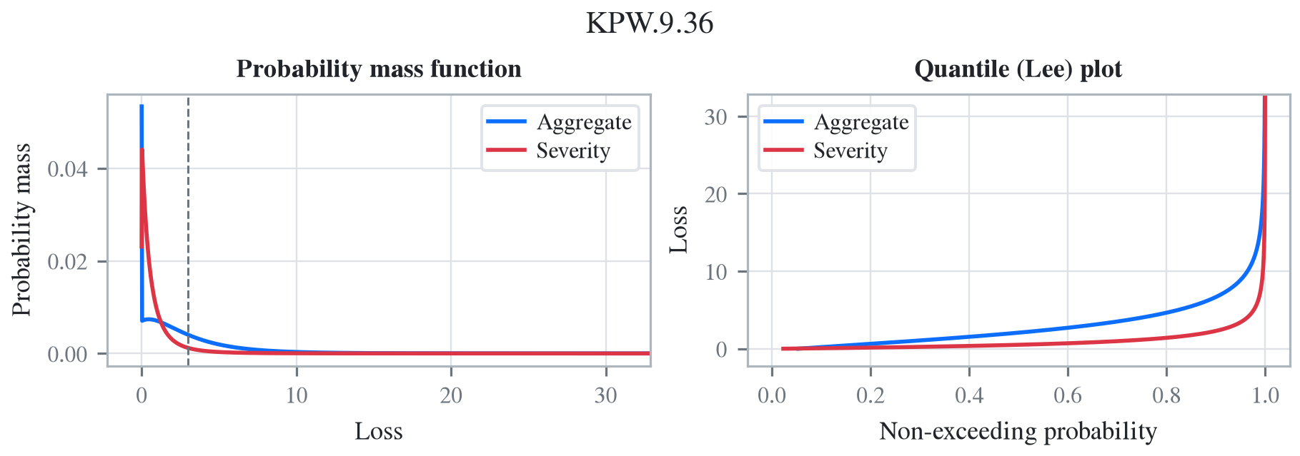
Exercise 9.36. The number of losses is Poisson with mean 3. Loss amounts have a Burr distribution with \(\alpha = 3\), \(\theta = 2\), and \(\gamma = 1\). Determine the variance of aggregate losses.
A matter of converting parameterizations. This is the scipy.statsburr12 distribution. The shape parameters are c=gamma and d=alpha. theta is a scale parameter.
Aggregate object: KPW.9.36. Frequency distribution poisson. Severity
burr12, [0, inf), power-law right tail. Updated with bucket size 1/32
and log2 = 16. Validation: fails sev cv, agg cv.

        Mean     SD      CV    Skew P01  Median    P99
X
Freq       3 1.7321 0.57735 0.57735
Sev  0.99994 1.7287  1.7288  21.773   0 0.53125 7.2812
Agg   2.9998 3.4591  1.1531  8.8756   0  2.0938 15.219
mean     = 3
variance = 12
std dev  = 3.4641
3 Compound Poisson, Example 9.9, 9.10
Policy A has a compound Poisson distribution with 2 expected claims and severity probabilities 0.6 on a payment of 1 and 0.4 on a payment of 2. Policy B has a compound Poisson distribution with 1 expected claim and probabilities 0.7 on a payment of 1 and 0.3 on a payment of 3.
Determine the probability that the total payment on the two policies will be 2.
p = build('port KPW.9.9.p ''agg A 2 claims dsev [1 2] [.6 .4] poisson ''agg B 1 claims dsev [1 3] [.7 .3] poisson')qd(p)
Portfolio object: KPW.9.9.p. Contains 2 aggregate components. Updated
with bucket size 1 and log2 = 6. Validation: not unreasonable.

            Mean      SD      CV    Skew P01 Median P99
unit  X
A     Freq     2  1.4142 0.70711 0.70711
      Sev    1.4  0.4899 0.34993 0.40825   1      1   2
      Agg    2.8  2.0976 0.74915 0.82344   0      2   9
B     Freq     1       1       1       1
      Sev    1.6 0.91652 0.57282 0.87287   1      1   3
      Agg    1.6  1.8439  1.1524  1.4037   0      1   7
total Agg    4.4  2.7928 0.63474 0.75284   0      4  12
Exercise 9.39. For a compound distribution, frequency has a binomial distribution with parameters m = 3 and q = 0.4 and severity has an exponential distribution with a mean of 100. Calculate \(\Pr(A \le 300)\).
Aggregate object: KPW.9.39. Frequency distribution binomial. Severity
expon, [0, inf), exponential right tail. Updated with bucket size 1/512
and log2 = 16. Validation: not unreasonable.

      Mean      SD      CV   Skew       P01  Median    P99
X
Freq   1.2 0.84853 0.70711 0.2357
Sev      1       1       1      2 0.0097656 0.69336 4.6055
Agg    1.2  1.3856  1.1547 1.7681         0 0.76172 6.0039
probability = 0.89413
Exercise 9.40. A company sells three policies. For policy A, all claim payments are 10,000 and a single policy has a Poisson number of claims with mean 0.01. For policy B, all claim payments are 20,000 and a single policy has a Poisson number of claims with mean 0.02. For policy C, all claim payments are 40,000 and a single policy has a Poisson number of claims with mean 0.03. All policies are independent. For the coming year, there are 5,000, 3,000, and 1,000 of policies A, B, and C, respectively. Calculate the expected total payment, the standard deviation of total payment, and the probability that total payments will exceed 30,000.
kpw_9_40 = build('port kpw_9_40\n''\tagg A 50 claims dsev [10] poisson\n''\tagg B 60 claims dsev [20] poisson\n''\tagg C 30 claims dsev [40] poisson\n')qd(kpw_9_40)qd(pd.Series({'expected payment': kpw_9_40.actual_m,'sd payment': kpw_9_40.actual_sd,'Pr > 3000': kpw_9_40.sf(3000)}).to_frame('value'), accuracy=5)
Portfolio object: kpw_9_40. Contains 3 aggregate components. Updated
with bucket size 10 and log2 = 9. Validation: not unreasonable.

            Mean     SD       CV    Skew  P01 Median  P99
unit  X
A     Freq    50 7.0711  0.14142 0.14142
      Sev     10      0        0           10     10   10
      Agg    500 70.711  0.14142 0.14142  340    500  670
B     Freq    60  7.746   0.1291  0.1291
      Sev     20      0        0           20     20   20
      Agg   1200 154.92   0.1291  0.1291  860   1200 1580
C     Freq    30 5.4772  0.18257 0.18257
      Sev     40      0        0           40     40   40
      Agg   1200 219.09  0.18257 0.18257  720   1200 1720
total Agg   2900 277.49 0.095686 0.11466 2280   2890 3570

                   value
expected payment    2900
sd payment        277.49
Pr > 3000        0.34658
4 Zero-Modified Binomial, Example 9.11
A compound distribution has a zero-modified binomial distribution with \(m = 3\), \(q = 0.3\), and \(p_0^M = 0.4\). Individual payments are 0, 50, and 150, with probabilities 0.3, 0.5, and 0.2, respectively. Use the recursive formula to determine the probability distribution of \(S\).
Solution.aggregate parameterizes the binomial by the per-trial probability q and the mean, so \(m = 3\) trials at \(q = 0.3\) is entered as \(mq = 0.9\) claims. That figure is the un-modified base mean: zm 0.4 then reweights the base binomial, exactly as in the \((a,b,1)\) construction of §6.6, and the realized \(\mathsf{E}(N)\) follows from it rather than being pinned to 0.9.
5 Extended Truncated Negative Binomial, Example 9.12
The number of claims has a Poisson–ETNB distribution with Poisson parameter \(\lambda = 2\) and ETNB parameters \(\beta = 3\) and \(r = 0.2\). The claim size distribution has probabilities 0.3, 0.5, and 0.2 at 0, 10, and 20, respectively. Determine the total claims distribution recursively.
NoteTo do
Needs a compound frequency with a zero-truncated secondary, a Poisson stopped sum of ZT negative binomials. Zero truncation itself is available since 1.0.0a152 (see Example 9.11), and here \(r = 0.2 > 0\), so this is an ordinary ZT negative binomial rather than the genuinely extended\(-1 < r < 0\) case. What is missing is the frequency-compounding slot: pascal is a Poisson stopped sum of an un-truncated negative binomial, and DecL has no way to zero-truncate the secondary distribution of a compound frequency. Tracked separately from [ZT-ZM-Frequency-Fix].
Exercise 9.45. For a compound Poisson distribution, has 6 expected claims and individual losses take values 1, 2, 4 with equal probabilities. Determine the distribution of the aggregate.
Exercise 9.47. Aggregate claims are compound Poisson with 2 expected claims and severity outcomes 1, 2 with probability 1/4 and 3/4. For a premium of 6, an insurer covers aggregate claims and agrees to pay a dividend (a refund of premium) equal to the excess, if any, of 75% of the premium over 100% of the claims. Determine the excess of premium over expected claims and dividends.
Aggregate object: KPW.9.47. Frequency distribution poisson. Severity
dhistogram, [1, 2], bounded; atoms [1 2]. Updated with bucket size 1 and
log2 = 5. Validation: not unreasonable.

      Mean      SD      CV    Skew P01 Median P99
X
Freq     2  1.4142 0.70711 0.70711
Sev   1.75 0.43301 0.24744 -1.1547   1      2   2
Agg    3.5  2.5495 0.72843 0.75429   0      3  11

            p       F        S  dividend
loss
0.0   0.13534 0.13534  0.86466       4.5
1.0  0.067668   0.203    0.797       3.5
2.0   0.21992 0.42292  0.57708       2.5
3.0   0.10432 0.52724  0.47276       1.5
4.0   0.17798 0.70522  0.29478       0.5
5.0  0.080391 0.78561  0.21439         0
6.0  0.095689  0.8813   0.1187         0
7.0  0.041288 0.92259 0.077408         0
8.0  0.038464 0.96106 0.038945         0
9.0    0.0159 0.97696 0.023045         0
prem      = 6
exp loss  = 3.5
dividend  = 1.6411
excess    = 0.85888
Exercise 9.57, 9.58. Aggregate losses have a compound Poisson claim distribution with 3 expected claims and individual claim amount distribution p(1) = 0.4, p(2) = 0.3, p(3) = 0.2, and p(4) = 0.1. Determine the probability that aggregate losses do not exceed 3.
Repeat the Exercise with a negative binomial frequency distribution with r = 6 and \(\beta = 0.5\).
Aggregate object: KPW.9.57. Frequency distribution poisson. Severity
dhistogram, [1, 4], bounded; atoms [1 2 3 4]. Updated with bucket size 1
and log2 = 6. Validation: not unreasonable.

      Mean     SD      CV    Skew P01 Median P99
X
Freq     3 1.7321 0.57735 0.57735
Sev      2      1     0.5     0.6   1      2   4
Agg      6  3.873  0.6455 0.75394   0      5  17
Aggregate object: KPW.9.58. Frequency distribution gamma. Severity
dhistogram, [1, 4], bounded; atoms [1 2 3 4]. Updated with bucket size 1
and log2 = 7. Validation: not unreasonable.

      Mean     SD      CV    Skew P01 Median P99
X
Freq     3 2.1213 0.70711 0.94281
Sev      2      1     0.5     0.6   1      2   4
Agg      6 4.5826 0.76376  1.0474   0      5  20

            Po                         NB
             p        F        S        p        F        S
loss
0.0   0.049787 0.049787  0.95021 0.087791 0.087791  0.91221
1.0   0.059744  0.10953  0.89047 0.070233  0.15802  0.84198
2.0   0.080655  0.19019  0.80981  0.08545  0.24348  0.75652
3.0   0.097981  0.28817  0.71183 0.095933  0.33941  0.66059
4.0    0.10751  0.39568  0.60432 0.098486  0.43789  0.56211
5.0    0.10445  0.50013  0.49987 0.089535  0.52743  0.47257
6.0   0.098668   0.5988   0.4012 0.082877  0.61031  0.38969
7.0   0.088215  0.68701  0.31299 0.073657  0.68396  0.31604
8.0    0.07506  0.76207  0.23793 0.063257  0.74722  0.25278
9.0   0.061311  0.82338  0.17662  0.05302  0.80024  0.19976
10.0  0.048587  0.87197  0.12803 0.043819  0.84406  0.15594
11.0  0.037239  0.90921  0.09079 0.035507  0.87957  0.12043
12.0  0.027715  0.93692 0.063075 0.028316  0.90789 0.092115
13.0  0.020101  0.95703 0.042974 0.022288  0.93017 0.069827
14.0  0.014239  0.97127 0.028735 0.017338  0.94751 0.052489
15.0 0.0098562  0.98112 0.018879 0.013334  0.96085 0.039155
Exercise 9.59. A policy covers physical damage incurred by the trucks in a company’s fleet. The number of losses in a year has a Poisson distribution with expectation 5. The amount of a single loss has a gamma distribution with shape 0.5 and scale 2,500. The insurance contract pays a maximum annual benefit of 20,000. Determine the probability that the maximum benefit will be paid. Use a span of 100 and the method of rounding.
V:\worktrees\aggregate_REFACTOR\src\aggregate\_bucket_window.py:1430: InfeasibleGridWarning: KPW.9.59: severity 'gamma' cannot be reproduced on this grid. The body needs bs <= 8.20968 (0.2102% of the mean is supplied below the first half bucket, and is placed at 0); the mean is not complete until the grid reaches 28,193, so matching it to 0.0001 needs log2 = 12, and log2 = 10 was used. A thick unlimited severity has this problem at any bucket size, because its mean is furnished far above its median and a finer bs only shortens the reach. Add an occurrence limit, or accept the reported moment errors. Further occurrences this session are suppressed; each object records its own verdict in validation.
  warn_infeasible_grid(agg)
Exercise 9.60. An individual has purchased health insurance, for which they pay 10 for each physician visit and 5 for each prescription. The probability that a payment will be 10 is 0.25, and the probability that it will be 5 is 0.75. The total number of payments per year has the Poisson–Poisson (Neyman Type A) distribution with primary mean 10 and secondary mean 4. Determine the probability that total payments in one year will exceed 400. Compare your answer to a normal approximation.
Aggregate object: KPW.9.60. Frequency distribution neyman. Severity
dhistogram, [5, 10], bounded; atoms [5 10]. Updated with bucket size 5
and log2 = 9. Validation: not unreasonable.

      Mean     SD      CV    Skew P01 Median P99
X
Freq    40 14.142 0.35355 0.41012
Sev   6.25 2.1651 0.34641  1.1547   5      5  10
Agg    250 89.443 0.35777 0.42101  70    245 485
FFT            0.054616
Normal approx  0.046766
6 Poisson Pareto, Example 9.14
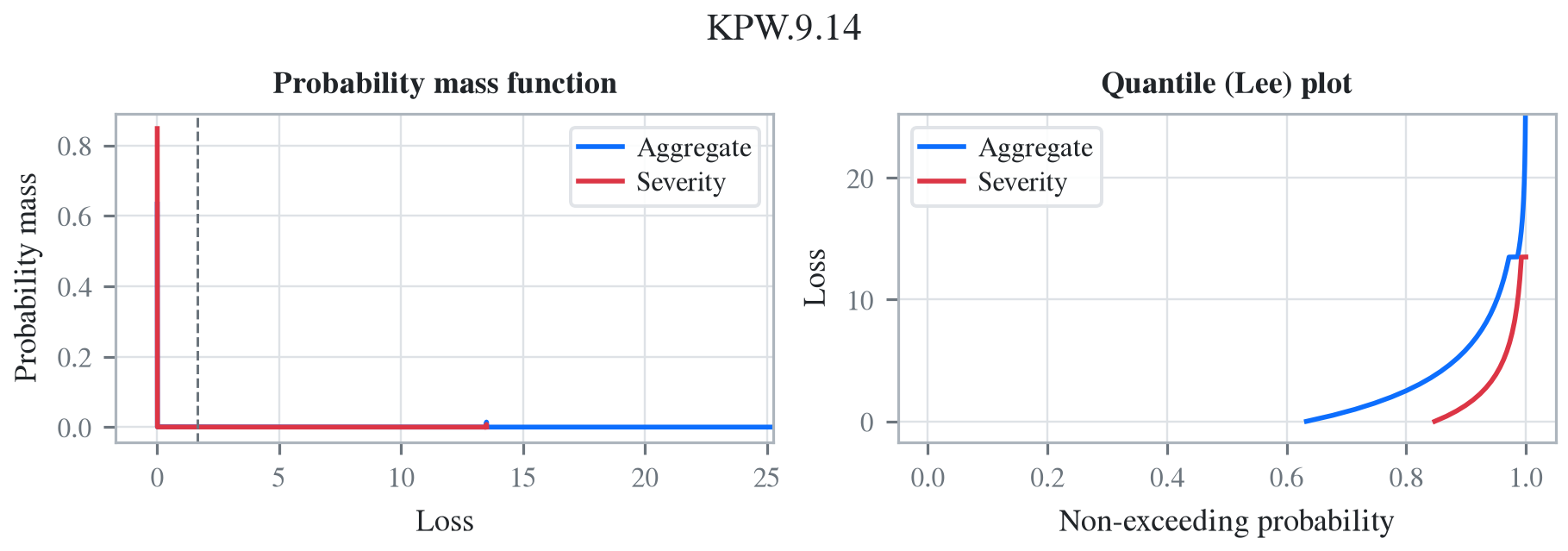
The number of ground-up losses is Poisson distributed with mean 3. The individual loss distribution is Pareto with shape parameter \(\alpha = 4\) and scale parameter 10. An individual ordinary deductible of 6, coinsurance of 75%, and an individual loss limit of 24 (before application of the deductible and coinsurance) are all applied. Determine the mean, variance, and distribution of aggregate payments.
The covered layer is 18 xs 6, in which the insured pays 25% because of the coinsurance clause. The severity is unconditional.
kpw_9_14 = build('agg KPW.9.14 3 claims ''18 xs 6 ''sev 10 * pareto 4 - 10 ! ''occurrence net of 25% po inf xs 0 ''poisson')qd(kpw_9_14)print(f'variance = {kpw_9_14.summary_df.loc["Agg", ["Mean", "CV"]].prod()**2:.6g}\ncomputed with bs=1/{1/kpw_9_14.bs:.0f} and log2={kpw_9_14.log2}')qd(kpw_9_14.density_df.loc[[0, 1, 2, 3], ['p', 'F', 'S']])kpw_9_14.plot();
Aggregate object: KPW.9.14. Frequency distribution poisson. Severity
pareto, [0, 18], bounded; 18 xs 6. Updated with bucket size 1/128 and
log2 = 16. Validation: reinsurance; subject not unreasonable.

        Mean     SD      CV    Skew P01 Median    P99
X
Freq       3 1.7321 0.57735 0.57735
Sev  0.54674 1.9199  3.5115  4.6513   0      0 11.719
Agg   1.6402 3.4575   2.108  2.8396   0      0 14.648
variance = 11.9546
computed with bs=1/128 and log2=16

              p       F       S
loss
0.0     0.63312 0.63312 0.36688
1.0  0.00051313 0.71515 0.28485
2.0  0.00038181 0.77526 0.22474
3.0  0.00033695 0.82028 0.17972
Under reinsurance summary_df reports the view the program requested, net here, as Mean / SD / CV / Skew on the Agg row; the gross figures it started from are the ('agg', 'subject', 'agg') row of reins_summary_df. The print statement computes net variance as the square of the product of the estimated mean and cv. The spikes on the density corresponds to the possibility of only limit claims.
Exercise 9.63. A ground-up model of individual losses has a gamma distribution with shape parameter 2 and scale 100. The number of losses has a negative binomial distribution with \(r = 2\) and \(\beta = 1.5\). An ordinary deductible of 50 and a loss limit of 175 (before imposition of the deductible) are applied to each individual loss.
Determine the mean and variance of the aggregate payments on a per-loss basis.
Determine the distribution of the number of payments.
Determine the cumulative distribution function of the amount of a payment, given that a payment is made.
Discretize the severity distribution using the method of rounding and a span of 40.
Calculate the discretized distribution of aggregate payments up to a discretized amount paid of 120.
Negative binomial \(c=1/2\) and hence mixing cv \(\sqrt{c}\), and the mean equals \(r\beta/(1+\beta)=1.4\). The cover is 125 xs 50. The severity is unconditional. First, the default calculation using bs=1/64.
The apparent difference in the severity distribution is caused by the rounding method. In the first case F(40) is almost exact whereas in the second it is actually F(60).
7 Group Life Individual Risk Model, Example 9.15, 9.18
Consider a group life insurance contract with an accidental death benefit. Assume that for all members the probability of death in the next year is 0.01 and that 30% of deaths are accidental. For 50 employees, the benefit for an ordinary death is 50,000 and for an accidental death it is 100,000. For the remaining 25 employees, the benefits are 75,000 and 150,000, respectively. Develop an individual risk model and determine its mean and variance.
Portfolio object: KPW.9.15.p. Contains 2 aggregate components. Updated
with bucket size 50 and log2 = 6. Validation: fails sev cv, agg cv.

             Mean      SD      CV     Skew P01 Median P99
unit  X
A     Freq    0.5 0.70356  1.4071   1.3929
      Sev      65  22.913 0.35251  0.87287  50     50 100
      Agg    32.5  48.517  1.4928   1.6562   0      0 200
B     Freq   0.25 0.49749    1.99   1.9699
      Sev    97.5  40.234 0.41265 0.090686  50    100 150
      Agg  24.375  52.512  2.1543   2.3721   0      0 200
total Agg  56.875  71.494   1.257   1.4575   0     50 300
mean     = 56.875
variance = 5001.984
std dev  = 70.7247
The density_df dataframe contains the exact aggregate distribution, which is not easy to compute by other means. KPW says (emphasis added)
With regard to calculating the probabilities, there are at least three options. One is to do an exact calculation, which involves numerous convolutions and almost always requires more excessive computing time. Recursive formulas have been developed, but they are cumbersome and are not presented here. For one such method, see De Pril [27]. One alternative is a parametric approximation as discussed for the collective risk model. Another alternative is to replace the individual risk model with a similar collective risk model and then do the calculations with that model. These two approaches are presented here.
The following solution attempts to commute convolution through the mixture. This works for a compound Poisson. However, the sum of binomials is not binomial, and so the frequencies can’t be independent binomial. They can be independent Poisson because it is additive.
        exact  compound Po      wrong
loss
0.0   0.47059      0.47237    0.47059
50.0      NaN      0.16533    0.16637
75.0      NaN     0.082664   0.083185
100.0     NaN     0.099787    0.10032
125.0     NaN     0.028932   0.029017
150.0     NaN     0.070835   0.071104
175.0     NaN     0.017463   0.017428
200.0     NaN     0.024881   0.024823
225.0     NaN     0.011552   0.011478
250.0     NaN     0.011399     0.0113
275.0     NaN    0.0040587  0.0039712
300.0     NaN    0.0050707   0.004986
325.0     NaN    0.0018166  0.0017595
350.0     NaN     0.001694  0.0016392
375.0     NaN   0.00077117 0.00073805
400.0     NaN   0.00064447 0.00061581
8 Group Life Individual Risk Model, Example 9.16, 9.17
A small manufacturing business has a group life insurance contract on its 14 permanent employees. The actuary for the insurer has selected a mortality table to represent the mortality of the group. Each employee is insured for the amount of his or her salary rounded up to the next 1,000. The group’s data are shown in the next table.
If the insurer adds a 45% relative loading to the net (pure) premium, what are the chances that it will lose money in a given year? Use the normal and lognormal approximations.
In order to make the answer self-contained, the code below includes the data munging to re-create the table, pasted from a pdf.
         Age Sex  Benefit       q
Employee
1         20   M    15000 0.00149
2         23   M    16000 0.00142
3         27   M    20000 0.00128
4         30   M    28000 0.00122
5         31   M    31000 0.00123
6         46   M    18000 0.00353
7         47   M    26000 0.00394
8         49   M    24000 0.00484
9         64   M    60000 0.02182
10        17   F    14000  0.0005
11        22   F    17000  0.0005
12        26   F    19000 0.00054
13        37   F    30000 0.00103
14        55   F    55000 0.00479
expected claim count = 0.04813
Here are the FFT-exact, and various approximations to the required probability. Working in thousands. The dsev clauses enter the fixed benefit amount for each employee. Note the outsize impact of employee 9.
from aggregate import Portfolioa = [build(f'agg ee.{i}{r.q} claims 'f'dsev [{r.Benefit /1000}] 'f'bernoulli')for i, r in df.iterrows()]kpw_9_16p = Portfolio('KPW.9.16p', a)kpw_9_16p.update(log2=8, bs=1, remove_fuzz=True)qd(kpw_9_16p)mv(kpw_9_16p)appx = kpw_9_16p.approximate('all')premium =1.45* kpw_9_16p.actual_mans = {k: v.sf(premium) for k, v in appx.items()}ans['FFT'] = kpw_9_16p.sf(premium)qd(pd.DataFrame(ans.values(), index=pd.Index(ans.keys(), name='method'), columns=['premium']).sort_values('premium'), accuracy=5)
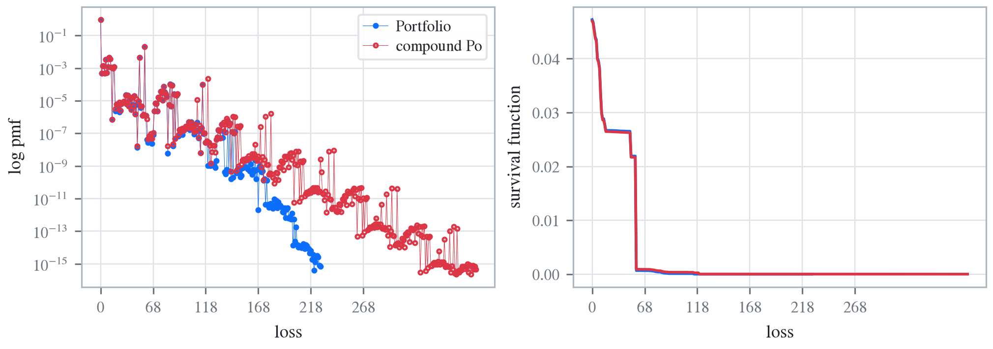
Here is a sample from the distribution and the mean-matched compound Poisson (for Exercise 9.18). The latter dsev clause works because all the benefit amounts are different. The temporary variable sev creates the severity curve. The log pmf graph reflects the irregular benefit amounts. Compare the cdf under comp Po with Table 9.17.
The insurance company reinsures amounts in excess of 100,000 on each life. The reinsurer wishes to charge a premium that is sufficient to guarantee that it will lose money 5% of the time on such groups. Obtain the appropriate premium by each of the following ways:
Using a normal approximation to the aggregate claims distribution.
Using a lognormal approximation.
Using a gamma approximation.
Using the compound Poisson approximation that matches the means.
In order to make the answer self-contained, the code below includes the data munging to re-create the table, pasted from a pdf.
Build the reinsurer’s loss distribution exactly, as p_ceded, a Portfolio, and the compound Poisson approximation cp_ceded, an Aggregate. The temporary variable bit is used to calculate the mixed severity distribution.
Exercise 9.74. A group insurance contract covers 1,000 employees. An employee can have at most one claim per year. For 500 employees, there is a 0.02 probability of a claim, and when there is a claim, the amount has an exponential distribution with mean 500. For 250 other employees, there is a 0.03 probability of a claim and amounts are exponential with mean 750. For the remaining 250 employees, the probability is 0.04 and the mean is 1,000. Determine the exact mean and variance of total claims payments. Next, construct a compound Poisson model with the same mean and determine the variance of this model.
kpw_9_74p = build('port KPW.9.74p ''agg A 10. claims sev 500 * expon binomial 0.02 ''agg B 7.5 claims sev 750 * expon binomial 0.03 ''agg C 10. claims sev 1000 * expon binomial 0.04 ')qd(kpw_9_74p)mv(kpw_9_74p)
Portfolio object: KPW.9.74p. Contains 3 aggregate components. Updated
with bucket size 2 and log2 = 16. Validation: not unreasonable.

            Mean     SD      CV    Skew  P01 Median   P99
unit  X
A     Freq    10 3.1305 0.31305 0.30666
      Sev    500    500       1       2    6    346  2302
      Agg   5000 2224.9 0.44497 0.66748  994   4750 11210
B     Freq   7.5 2.6972 0.35963 0.34851
      Sev    750    750       1       2    8    520  3454
      Agg   5625 2882.9 0.51251 0.76882  686   5252 13864
C     Freq    10 3.0984 0.30984 0.29693
      Sev   1000   1000       1       2   10    694  4606
      Agg  10000 4427.2 0.44272 0.66417 2014   9506 22348
total Agg  20625 5732.4 0.27794 0.44276 9214  20202 35772
mean     = 20625
variance = 3.286094e+07
std dev  = 5732.45
Compound Poisson approximation is easy to construct as a mixture.
Aggregate object: KPW.9.74.cp. Frequency distribution poisson. Mixed
severity with 3 components. Updated with bucket size 2 and log2 = 16.
Validation: not unreasonable.

      Mean     SD      CV    Skew  P01 Median   P99
X
Freq  27.5  5.244 0.19069 0.19069
Sev    750 808.34  1.0778   2.372    6    492  3804
Agg  20625 5782.5 0.28036 0.44729 9134  20194 35922
mean     = 20625
variance = 3.34375e+07
std dev  = 5782.52
Programs in the aggregate Loss Lab
Each program below opens in the aggregate Loss Lab, which builds it with nothing to install. The names are those in recitations.agg, where every program is renamed by its text’s citation key, or by Exam for an examination question.
Klugman2019.KPW.95: Examples 9.5 and 9.6, group dental payments per employee.