Brehm et al. on reinsurance in enterprise risk analysis

Brehm, Perry, Venter and Witcraft (2007), Enterprise Risk Analysis for Property and Liability Insurance Companies, Section 2.5

Author

Stephen J. Mildenhall

Published

2026-10-22 19:57 commit b7145b5+

This section re-analyzes reinsurance structure alternatives introduced in Brehm et al. (2007), Enterprise Risk Analysis for Property & Liability Insurance Companies. This book is the ERM text on the syllabus for CAS Exam Part 7.

1 Reinsurance Example

This section analyzes the example given in Section 2.5 of Enterprise Risk Analysis.

Assumptions. ABCD writes 33M excess property and casualty business.

ABCD total gross
- Loss ratio: 69.36%
- Expense ratio: 23%
- Combined ratio: 92.36%
- Margin 2.52M
Casualty
- 14M premium
- 78% expected loss ratio
- 5M limits
- 4M xs 1M reinsurance, ceded premium 4.41M
Property
- 19M premium
- 63% expected loss ratio
- 20M limits
- 17M xs 3M per risk reinsurance, ceded premium 2.36M
- 95% share of 24M xs 1M cat reinsurance, ceded premium 1.53M with 1@100%
- Cat program designed to cover to 250-year event.
Reinsurance total
- Average recoveries 5.08M
- Ceded premium 8.3M
- Net premium 24.7M
Mythical alternative program
- Stop-loss, 20 xs 30, ceded premium 1.98

Additional assumptions. There are no details of the stochastic model, so we assume

Frequency and severity models per DecL below,
Split the property losses into cat and non-cat by assuming that cat premium equals 2M, non-cat premium 17M, at the same loss ratios (this is just a split of losses, the by line loss ratios are not used), and
Cat, non-cat and casualty are independent.
Free and unlimited reinstatements on the catastrophe protection. See REF for a discussion of reinstatements.

2 Stochastic Models and Baseline Analysis

Construct the gross and net portfolios. All amounts in millions.

2.1 Gross Portfolio

The 250-year cat PML is printed last, to compare with the 25M program.

from aggregate import qd, mv
import pandas as pd
import matplotlib.pyplot as plt

abcd = build('port ABCD '
         'agg Casualty 14.0 premium at 78% lr '
             '5 xs 0 '
             'sev lognorm 0.1 cv 10 '
             'mixed gamma 0.3 '
         'agg PropertyNC 17.0 premium at 63% lr '
             '25 xs 0 '
             'sev lognorm [0.1 1] cv [5 10] wts [.7 .3] '
             'mixed gamma 0.1 '
         'agg PropertyC 2.0 premium at 63% lr '
             '150 xs 0 '
             'sev 3 * pareto 2.375 - 3 '
             'poisson ', bs=1/128)
qd(abcd)
mv(abcd)
print(abcd['PropertyC'].q(0.996))

Portfolio object: ABCD. Contains 3 aggregate components. Updated with
bucket size 1/128 and log2 = 16. Validation: fails sev mean, agg mean.

                    Mean      SD      CV    Skew      P01    Median    P99
unit       X                                                              
Casualty   Freq   125.93  39.409 0.31296 0.60054                          
           Sev  0.086436 0.34822  4.0286  9.5552        0 0.0078125 1.4766
           Agg    10.885  5.1839 0.47626 0.88565   2.4844    10.102 26.102
PropertyNC Freq   34.918  6.8638 0.19657 0.24744                          
           Sev   0.30659   1.506  4.9121  11.569        0   0.03125 5.4531
           Agg    10.706  9.1446 0.85419  1.9358   1.4531    7.5938 42.375
PropertyC  Freq   0.5801 0.76165  1.3129  1.3129                          
           Sev     2.172  4.3889  2.0207  11.511 0.015625    1.0156 17.859
           Agg      1.26  3.7298  2.9601  12.398        0         0 14.867
total      Agg     22.85  11.154 0.48813  1.6193   7.0234    20.375 58.766
mean     = 22.89
variance = 124.4768
std dev  = 11.1569
22.859375

2.2 Net Portfolio

abcd_net = build('port ABCD:Net '
         'agg Casualty 14.0 premium at 78% lr '
             '5 xs 0 '
             'sev lognorm 0.1 cv 10 '
             'occurrence net of 4 xs 1 '
             'mixed gamma 0.3 '
         'agg PropertyNC 17.0 premium at 63% lr '
             '25 xs 0 '
             'sev lognorm [0.1 1] cv [5 10] wts [.7 .3] '
             'occurrence net of 17 xs 3 '
             'mixed gamma 0.1 '
         'agg PropertyC 2.0 premium at 63% lr '
             '150 xs 0 '
             'sev 3 * pareto 2.375 - 3 '
             'occurrence net of 24 xs 1 '
             'poisson ', bs=1/128)
qd(abcd_net)
qd(abcd_net.est_sd)

Portfolio object: ABCD:Net. Contains 3 aggregate components. Updated
with bucket size 1/128 and log2 = 16. Validation: reinsurance; subject
fails sev mean, agg mean.

                    Mean      SD      CV    Skew      P01    Median    P99
unit       X                                                              
Casualty   Freq   125.93  39.409 0.31296 0.60054                          
           Sev  0.065564   0.166  2.5318  4.1715        0 0.0078125      1
           Agg    8.2563  3.1853  0.3858 0.65534   2.4375    7.9062 17.141
PropertyNC Freq   34.918  6.8638 0.19657 0.24744                          
           Sev    0.2098 0.60011  2.8604  6.1847        0   0.03125      3
           Agg    7.3259  3.8274 0.52244  1.0361   1.4531    6.6641 18.984
PropertyC  Freq   0.5801 0.76165  1.3129  1.3129                          
           Sev   0.80417   2.199  2.7345  36.228 0.015625         1      1
           Agg    0.4665  1.7834  3.8228  40.649        0         0    2.5
total      Agg    16.049  5.2892 0.32957  2.0938    6.625    15.484 30.305
5.2892

2.3 Ceded Portfolio

abcd_ceded = build('port ABCD:Ceded '
         'agg Casualty 14.0 premium at 78% lr '
             '5 xs 0 '
             'sev lognorm 0.1 cv 10 '
             'occurrence ceded to 4 xs 1 '
             'mixed gamma 0.3 '
         'agg PropertyNC 17.0 premium at 63% lr '
             '25 xs 0 '
             'sev lognorm [0.1 1] cv [5 10] wts [.7 .3] '
             'occurrence ceded to 17 xs 3 '
             'mixed gamma 0.1 '
         'agg PropertyC 2.0 premium at 63% lr '
             '150 xs 0 '
             'sev 3 * pareto 2.375 - 3 '
             'occurrence ceded to 24 xs 1 '
             'poisson ', bs=1/128)
qd(abcd_ceded)
qd(abcd_ceded.est_sd)

Portfolio object: ABCD:Ceded. Contains 3 aggregate components. Updated
with bucket size 1/128 and log2 = 16. Validation: reinsurance; subject
fails sev mean, agg mean.

                    Mean      SD      CV    Skew P01   Median     P99
unit       X                                                         
Casualty   Freq   125.93  39.409 0.31296 0.60054                     
           Sev  0.020872 0.23387  11.205  14.019   0        0 0.47656
           Agg    2.6283  2.7503  1.0464  1.3572   0   1.7578  11.461
PropertyNC Freq   34.918  6.8638 0.19657 0.24744                     
           Sev  0.096787  1.0315  10.657   13.51   0        0  2.4531
           Agg    3.3796  6.1312  1.8142  2.3095   0        0  25.344
PropertyC  Freq   0.5801 0.76165  1.3129  1.3129                     
           Sev    1.3679  3.0831   2.254  4.2512   0 0.015625  16.859
           Agg    0.7935   2.569  3.2375  5.6851   0        0  13.312
total      Agg    6.8014  7.1941  1.0577  1.7643   0   4.4844  31.516
7.1941

2.4 Reinsurance Summary

The bottom table shows expected losses, counts, severity, loss ratios and margins implicit in the given reinsurance structure, pricing, and the gross stochastic model. implicit in the given reinsurance structure, pricing, and the gross stochastic model. The non-cat property reinsurance has the highest ceded loss ratio and the cat program the lowest.

Note

This summary previously used the per-unit, per-layer reinsurance_occ_layer_df dataframe, removed in 1.0.0a19 in favour of the whole-structure reins_summary_df / reins_stats_df / reins_density_df objects. To rebuild it, take each unit’s ceded occurrence aggregate mean and CV from the ('occ', 'ceded', 'agg') row of reins_summary_df, columns Est EX and Est CV, as the layer loss cost ex and cv; the ceded count is unit.n * unit.sev.sf(attach). Combine with the given premium to form the loss ratio and margin. For a per-layer split, build each layer as its own occurrence cover.

2.5 Underwriting Result Distributions

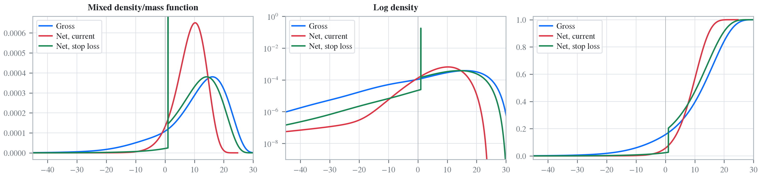
Make the underwriting result distributions, including the proposed stop loss reinsurance (computed by hand). The dataframe compare accumulates the gross, ceded, and net probability mass functions. We use these to determine statistics and to plot.

compare = abcd.density_df[['loss', 'p_total']]; \
compare.columns = ['loss', 'gross']; \
compare['gross_uw'] = 33 - compare.loss; \
compare['net_current'] = abcd_net.density_df.p_total; \
compare['net_current_uw'] = 33 - 4.41 - 2.36 - 1.53 - compare.loss;
from aggregate.distributions import make_ceder_netter
compare['net_stoploss'] = abcd.density_df.p_total; \
c, n = make_ceder_netter([(1, 20, 30)]); \
compare['nsll'] = n(compare.loss); \
g = compare.groupby('nsll').net_stoploss.sum(); \
compare['net_stoploss'] = 0.0; \
compare.loc[g.index, 'net_stoploss'] = g; \
compare['net_stoploss_uw'] = 33 - 1.98 - compare.loss;

2.6 Comparison with the Book’s Figures

Statistics summary, compare Figure 2.5.2.

from aggregate import MomentWrangler
from scipy.interpolate import interp1d
ans = []; cdfs = []
for xs, den in [(compare.gross_uw, compare.gross), (compare.net_current_uw, compare.net_current),
                 (compare.net_stoploss_uw, compare.net_stoploss)]:
    xd = xs * den
    ex1 = np.sum(xd)
    xd *= xs
    ex2 = np.sum(xd)
    ex3 = np.sum(xd * xs)
    mw = MomentWrangler()
    mw.noncentral = ex1, ex2, ex3
    ans.append(mw)
    cdfs.append(interp1d(den.cumsum(), xs))

fig_252 = pd.concat([i.stats for i in ans], keys=['Gross', 'Current', 'StopLoss'], axis=1)
for p in [0.01, 0.99]:
    fig_252.loc[f'q({p})'] = [float(i(p)) for i in cdfs]
qd(fig_252)


          Gross  Current  StopLoss
ex        10.15   8.6513    10.021
var      124.41   27.975    58.777
sd       11.154   5.2892    7.6666
cv       1.0989  0.61137   0.76502
skew    -1.6193  -2.0938   -1.0088
q(0.01)   25.98   18.081        24
q(0.99)  -25.76  -5.6036   -7.7399

Plot of densities and distributions, compare Figure 2.5.3 and 2.5.4.

fig, axs = plt.subplots(1, 3, figsize=(3 * 3.5, 2.45), constrained_layout=True)
ax0, ax1, ax2 = axs.flat

for ax in [ax0, ax1]:
    ax.plot(compare.gross_uw, compare.gross, label='Gross')
    ax.plot(compare.net_current_uw, compare.net_current, label='Net, current')
    yl = ax.get_ylim()
    ax.plot(compare.net_stoploss_uw, compare.net_stoploss, label='Net, stop loss')
    ax.legend(loc='upper left')
    ax.set(xlim=[-45, 30], ylim=yl)
    ax.axvline(0, lw=.25, c='C7')
ax1.set(yscale='log', ylim=[1e-9, 1], title='Log density'); \
ax0.set(title='Mixed density/mass function');

ax2.plot(compare.gross_uw, 1 - compare.gross.cumsum(), label='Gross'); \
ax2.plot(compare.net_current_uw, 1 - compare.net_current.cumsum(), label='Net, current'); \
ax2.plot(compare.net_stoploss_uw, 1 - compare.net_stoploss.cumsum(), label='Net, stop loss'); \
ax2.legend(loc='upper left'); \
ax2.set(xlim=[-45, 30], ylim=[-0.025, 1.025]);
ax2.axvline(0, lw=.25, c='C7');

Numerical distribution of underwriting results at various return points, compare Figure 2.5.5. Given there was no information about the stochastic model provided, and the model here is based on common benchmarks, the agreement between the two distributions is striking.

fig_255 = pd.DataFrame(columns=['Gross', 'Current', 'StopLoss'], dtype=float)

for p in [.0025, .005, 0.0075, .01, .0125, .015, .0175, .02,
          .04, .06, .08, .1, .12, .14, .16, .18, .2, .22, .24,
          .25, .26, .28, .3, .32, .34, .36, .38, .4, .42, .44,
          .46, .48, .5]:
    fig_255.loc[p] = [float(i(1-p)) for i in cdfs]
fig_255.index.name = 'p'
qd(fig_255, float_format=lambda x: f'{x:.3f}', max_rows=len(fig_255))


         Gross  Current  StopLoss
p                                
0.0025 -38.503  -10.257   -20.483
0.0050 -32.113   -7.826   -14.093
0.0075 -28.394   -6.514   -10.374
0.0100 -25.760   -5.604    -7.740
0.0125 -23.740   -4.902    -5.720
0.0150 -22.114   -4.328    -4.094
0.0175 -20.758   -3.842    -2.738
0.0200 -19.595   -3.420    -1.575
0.0400 -13.603   -1.182     1.021
0.0600  -9.962    0.182     1.021
0.0800  -7.211    1.186     1.022
0.1000  -4.936    1.991     1.023
0.1200  -2.978    2.669     1.024
0.1400  -1.263    3.259     1.025
0.1600   0.246    3.784     1.026
0.1800   1.575    4.259     1.027
0.2000   2.752    4.695     1.028
0.2200   3.801    5.100     1.821
0.2400   4.745    5.478     2.765
0.2500   5.183    5.659     3.203
0.2600   5.603    5.835     3.623
0.2800   6.391    6.173     4.411
0.3000   7.121    6.496     5.141
0.3200   7.802    6.805     5.822
0.3400   8.442    7.103     6.462
0.3600   9.047    7.390     7.067
0.3800   9.622    7.669     7.642
0.4000  10.171    7.941     8.191
0.4200  10.697    8.206     8.717
0.4400  11.203    8.465     9.223
0.4600  11.692    8.720     9.712
0.4800  12.167    8.970    10.187
0.5000  12.628    9.217    10.648

Programs in the aggregate Loss Lab

Each program below opens in the aggregate Loss Lab, which builds it with nothing to install. The names are those in recitations.agg, where every program is renamed by its text’s citation key, or by Exam for an examination question.

Brehm2007.ABCD: Section 2.5, the gross portfolio of the reinsurance example.
Brehm2007.ABCD:Net: Section 2.5, the same portfolio net of the reinsurance program.
Brehm2007.ABCD:Ceded: Section 2.5, the reinsurance program ceded from the portfolio.

Brehm, P. J., Perry, J. H., Venter, G. G., & Witcraft, S. E. (2007). Enterprise Risk Analysis. Casualty Actuarial Society.