Using PricingBounds

Exact price ranges of other risks over all distortions that price a reference risk to a given premium

When a portfolio \(X\) with assets \(a\) is priced to a premium \(P\), the pricing distortion is not known, only that it is one of the set \(G_P\) of distortions \(g\) with \(g[X \wedge a] = P\). Square brackets mark \(g\) acting on a random variable, as a spectral risk measure, and parentheses mark \(g\) acting on a probability. The class PricingBounds¹ computes the range of the price \(g[Y]\) of another risk \(Y\), such as a reinsurance layer, over every \(g\) in \(G_P\). The narrower the range, the more closely the price of \(X\) determines the price of \(Y\).

A distortion \(g\) with Kusuoka measure \(\mu\) prices any risk \(Z\) by \(g[Z] = \int \mathrm{TVaR}_p(Z)\,\mu(dp)\). The premium of \(X\) and the price of \(Y\) are both linear in \(\mu\), so the extreme prices are attained by biTVaRs, mixtures of two TVaRs. As \(p\) runs over \([0, 1]\) the point \((\mathrm{TVaR}_p(X), \mathrm{TVaR}_p(Y))\) traces a curve, a biTVaR prices \(X\) and \(Y\) at a point on a chord of the curve, and the range of the price of \(Y\) is the vertical slice at \(\mathrm{TVaR}_X = P\) through the convex hull of the curve. Between consecutive CDF breakpoints of \(X\) and \(Y\) both TVaRs are affine in \(1/(1-p)\), so on the discrete grid the curve is exactly piecewise linear, with vertices at the union of the breakpoints, and the bounds are exact. With finite \(a\) both risks are capped at \(a\).

The envelope of the distortions in \(G_P\), computed by Bounds (Using Bounds), also bounds the price of \(Y\), but not sharply, and PricingBounds computes the exact range. It is a subclass of the same convex hull engine as AllocationBounds (Using AllocationBounds), which bounds the share of \(P\) allocated to each unit of a portfolio. Use PricingBounds for the price of a risk on its own, AllocationBounds for a unit’s share of the portfolio premium, and Bounds for the distortions themselves. The hull is computed once, and bounds(P) slices it at any premium in premium_range.

from aggregate.bounds import PricingBounds
PricingBounds(x_source, y_sources, a=np.inf, s_floor=1e-14)
port.pricing_bounds(y_sources, a=0, p=0)     # the total of port is x_source

The reference x_source is an Aggregate, a Portfolio (its total), a PnL (its loss engine), a probability Series indexed by outcome, or 'uniform'. The argument y_sources is one such risk, a list of them, or a dictionary from names to risks. The method Portfolio.pricing_bounds sets \(a\) from a, or from a probability p as \(a = q(p)\), and with both zero leaves the risks uncapped.

import numpy as np
import pandas as pd
from aggregate import build, __version__
from aggregate.bounds import PricingBounds
from style import wprint, GT, refuse, figures, figure
figures()
print(__version__)

2.1.0a5

Aggregate layers on a portfolio

The example is the portfolio Two of Using Bounds. Unit Thin has 10 claims with a gamma severity of mean 10 and CV 0.5, and unit Thick has 2 claims with a lognormal severity of mean 20 and CV 2, limited to 250. Assets are the 99th percentile of the total, \(a = 365.125\), and the premium \(P = 158.797\) earns a 10% cost of capital. The risks to price are two aggregate layers on the total, 50 xs 150 and 100 xs 250, built as probability series from density_df, and the total itself, under the name Two.

port = build('''port Two
  agg Thin  10 claims sev gamma 10 cv 0.5 poisson
  agg Thick  2 claims 250 xs 0 sev lognorm 20 cv 2 poisson''')
a = port.q(0.99)
port.calibrate_distortions(0.10, a=a)
P = port.calibration_df.P.iloc[0]
x = port.density_df.loss
layers = {f'{l} xs {r}': port.density_df.p_total.groupby(np.clip(x - r, 0, l)).sum()
          for r, l in [(150, 50), (250, 100)]}
pb = PricingBounds(port, {**layers, 'Two': port}, a=a)
wprint(pb)
GT(pb.bounds(P).droplevel('P'), float_format='.3f')

PricingBounds(X='X', Y=['50 xs 150', '100 xs 250', 'Two'], a=365.125, 8243
vertices, premium range [138.164, 365.125])

risk	lower	upper	width
100 xs 250	3.810	11.811	8.000
50 xs 150	14.098	18.497	4.399
Two	158.797	158.797	0.000

The feasible premiums run from \(L = \mathsf{P}(X \wedge a) = 138.164\) to \(a\). At \(P\) the price of 50 xs 150 lies between 14.098 and 18.497, and the price of 100 xs 250 between 3.810 and 11.811, an upper end about three times the lower. The total has the single price \(P\), because every distortion in \(G_P\) prices it to \(P\).

Each of the five calibrated distortions (see Using distortions) is in \(G_P\), so its price of each layer lies in the range. The table lists them in order of their Gini index, gini. The tvar distortion attains the lower bound on 100 xs 250. On 50 xs 150 the largest calibrated price, 16.245 from ph, is well short of the upper bound.

prices = pd.DataFrame({n: {k: d.price(y).ask for k, d in port.distortions.items()}
                       for n, y in layers.items()})
prices.insert(0, 'gini', port.distortion_df.gini)
GT(prices.rename_axis('distortion'), float_format='.3f', formatters={'gini': '{x:.4f}'})

distortion	gini	50 xs 150	100 xs 250
ccoc	0.0909	14.405	11.702
ph	0.1556	16.245	7.359
wang	0.1868	16.218	5.813
dual	0.2196	15.791	4.447
tvar	0.2461	14.386	3.810

Distortions that attain the pricing bounds

The method bitvars(P) lists the biTVaR at each end of each range, as p0, p1, and the weight w1 on p1. The upper bound on 100 xs 250 mixes the mean, \(p_0 = 0\), with TVaR at 0.985, with weight 0.093. It is close to the ccoc distortion, which mixes the mean with the maximum. The lower bound is a bracket around \(p^* = 0.2461\), equivalent to TVaR at \(p^*\). The method distortion(P, risk, bound) returns the achieving Distortion, and check(P) reprices each risk and the total from first principles with it. The largest errors are below \(10^{-11}\).

print(pb.distortion(P, '100 xs 250', 'upper'))
print(pb.check(P)[['err', 'total_err']].abs().max().to_dict())
GT(pb.bitvars(P).droplevel('P'), float_format='.4f')

bitvar(0, 0.98496; 0.09266)
{'err': 4.2454928461665986e-13, 'total_err': 5.4285465012071654e-12}

risk	bound	value	p0	p1	w1
100 xs 250	lower	3.8102	0.2457	0.2462	0.9083
	upper	11.8107	0.0000	0.9850	0.0927
50 xs 150	lower	14.0979	0.1202	0.9900	0.0470
	upper	18.4966	0.0000	0.7868	0.2283
Two	lower	158.7969	0.0000	0.9900	0.0909
	upper	158.7969	0.0000	0.9900	0.0909

Bounds as the premium varies

The hull does not depend on the premium, so bounds accepts a list of premiums at almost no cost. The width of each range is zero at \(L\), where only the identity distortion \(g(s) = s\) prices \(X \wedge a\) to \(L\), and it grows with the premium. The plot shows the curve of each layer against \(\mathrm{TVaR}_p(X)\), its lower and upper hulls, and the slice at \(P\).

Ps = [pb.premium_range[0], 145, 150, P, 170, 200]
GT(pb.bounds(Ps).width.unstack(), float_format='.3f')

P	100 xs 250	50 xs 150	Two
138.164	0.000	0.000	0
145.000	2.726	1.647	0
150.000	4.670	2.667	0
158.797	8.000	4.399	0
170.000	12.066	6.604	0
200.000	21.720	12.508	0

fig, axs = figure('full', cols=2)
pb.plot(items=list(layers), P=P, axs=axs);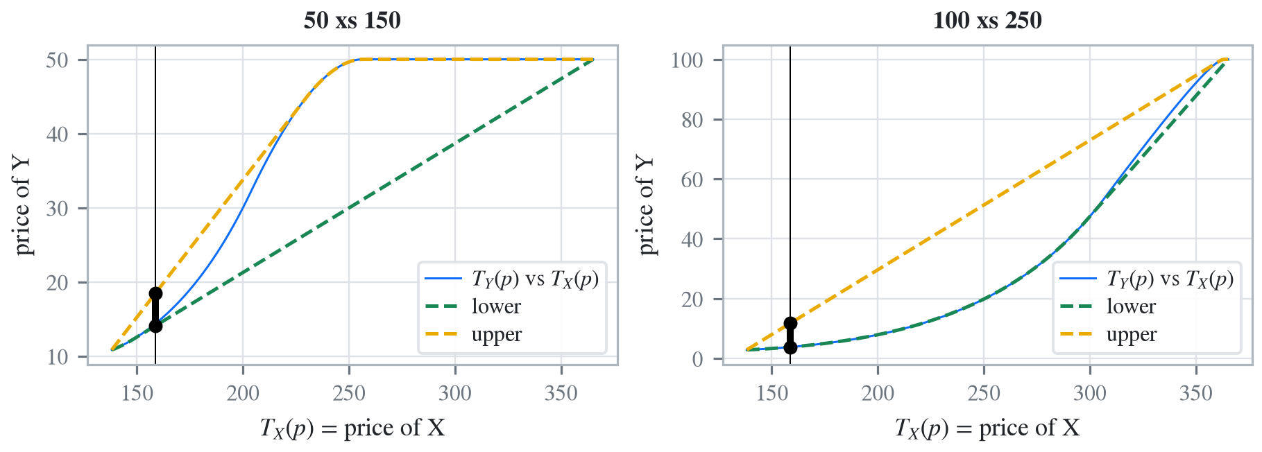

The curve of 50 xs 150 is flat at 50 for \(p \ge \Pr(X < 200) = 0.871\), where \(\mathrm{TVaR}_X = 256.6\), because every outcome in the tail then exhausts the layer. At \(P\) the curve of 100 xs 250 lies on its lower hull, so the lower bound is TVaR at \(p^*\), and its upper hull is far above the curve.

The uniform reference and the Gini index

With x_source='uniform' the reference is the uniform distribution on \([0, 1]\), with \(\mathrm{TVaR}_p = (1 + p)/2\). A distortion prices it at \(\int_0^1 g(s)\,ds\), the area under \(g\), so a premium \(P\) for the uniform fixes the Gini index of \(g\) at \(2P - 1\), the gini column of distortion_df. In Kusuoka terms \(2P - 1 = \int p\,\mu(dp)\), the mean TVaR level, which mean_kusuoka_level(P) returns. The bounds are the range of the price of \(Y\) over all distortions with a given Gini index. The table shows the range of the price of the total of Two at the Gini index of each calibrated distortion. Each range contains 158.797, the price of the total under every calibrated distortion: ccoc is near the top of its range and tvar near the bottom.

gl = PricingBounds('uniform', {'Two': port}, a=a)
gini = port.distortion_df.gini
GT(pd.DataFrame({k: gl.bounds((1 + g) / 2).iloc[0] for k, g in gini.items()}).T
   .assign(gini=gini)[['gini', 'lower', 'upper', 'width']]
   .rename_axis('distortion'), float_format='.4f')

distortion	gini	lower	upper	width
ccoc	0.0909	145.7791	159.0098	13.2307
ph	0.1556	151.1997	173.8484	22.6487
wang	0.1868	153.8115	180.9983	27.1867
dual	0.2196	156.5622	188.5280	31.9659
tvar	0.2461	158.7814	194.6031	35.8217

Refused inputs

A premium outside premium_range is refused, and so is a call to mean_kusuoka_level when the reference is not the uniform.

refuse(lambda: pb.bounds(400), lambda: pb.mean_kusuoka_level(P))

P=[400.] outside feasible premium range [138.164, 365.125] (= [E[X], TVaR at
s_floor truncation]).
mean_kusuoka_level requires the uniform X-source (pass x_source='uniform').

Footnotes

1. From aggregate 1.0