Using Bounds

Pricing bounds: the envelope of all distortions that price a risk to a given premium with given assets

A premium \(P\) for a risk \(X\) supported by assets \(a\) does not determine the pricing distortion. Any distortion \(g\) with \[ g[X \wedge a] = \int_0^a g(S(x))\,dx = P, \] where \(S\) is the survival function of \(X\), is consistent with it. Square brackets mark \(g\) acting on a random variable, as a spectral risk measure, and parentheses mark \(g\) acting on a probability. The class Bounds computes the set \(G_P\) of these distortions and its envelope: the smallest and largest value of \(g(s)\) at each \(s\) over \(G_P\). The method is from Mildenhall (2022), “Similar risks have similar prices: a useful and exact quantification”, Insurance: Mathematics and Economics 105.

Every concave distortion is a mixture of TVaR distortions, \(g(s) = \int \min(1, s/(1-p))\,\mu(dp)\), and then \(g[X \wedge a] = \int \mathrm{TVaR}_p(X \wedge a)\,\mu(dp)\). The premium is one linear condition on \(\mu\), so the extreme points of \(G_P\) are biTVaRs, \[ g = (1-w)\,\mathrm{TVaR}_{p_0} + w\,\mathrm{TVaR}_{p_1}, \qquad p_0 \le p^* < p_1, \] where \(\mathrm{TVaR}_{p^*}(X \wedge a) = P\) and the weight \(w\) makes \(g\) price \(X \wedge a\) to \(P\). The class Bounds evaluates every bracket \((p_0, p_1)\) from a grid of 256 values of \(p\), refined near \(p^*\), at 513 values of \(s\). A minimum of concave functions is concave, so the lower edge, min_envelope, is a Distortion. The upper edge, max_envelope, is not concave in general and is a plain function of \(s\).

The class Bounds is one of three classes in aggregate.bounds¹. It computes the set \(G_P\) itself, for one premium fixed when it is built. The class PricingBounds computes the exact range of the price of another risk over \(G_P\) (Using PricingBounds), and AllocationBounds the range of the natural allocation of \(P\) to each unit of a portfolio (Using AllocationBounds). Those two are subclasses of one convex hull engine and take the premium at call time. Use Bounds to see which distortions are admissible, and the other two for the price of a particular risk or unit.

from aggregate.bounds import Bounds
Bounds(obj, premium, a=np.inf, unit='total', n_p=256, n_s=513)

The risk obj is a Portfolio (its total, or the unit given by unit), an Aggregate, a PnL (its loss engine), or a probability Series indexed by outcome. The premium must lie between the mean of \(X\) and \(a\).

import numpy as np
import pandas as pd
from aggregate import build, __version__
from aggregate.bounds import Bounds, PricingBounds
from style import wprint, GT, refuse, figures
figures()
print(__version__)

2.0.0

A two-unit portfolio priced at a 10% cost of capital

The example here, and on the pages for PricingBounds and AllocationBounds, is the portfolio Two. Unit Thin has 10 claims a year with a gamma severity of mean 10 and coefficient of variation (CV) 0.5, and unit Thick has 2 claims with a lognormal severity of mean 20 and CV 2, limited to 250. Assets are the 99th percentile of the total, \(a = 365.125\). The method calibrate_distortions sets the premium that earns a 10% cost of capital on \(Q = a - P\), so that \(P = L + 0.1(a - P)\) with expected loss \(L = \mathsf{P}(X \wedge a)\), and calibrates the five standard distortions to it (see Using distortions).

port = build('''port Two
  agg Thin  10 claims sev gamma 10 cv 0.5 poisson
  agg Thick  2 claims 250 xs 0 sev lognorm 20 cv 2 poisson''')
a = port.q(0.99)
port.calibrate_distortions(0.10, a=a)
P = port.calibration_df.P.iloc[0]
GT(port.calibration_df[['L', 'M', 'P', 'Q', 'a']], float_format=',.3f')

unit	L	M	P	Q	a
calibration	138.164	20.633	158.797	206.328	365.125

The premium is \(P = 158.797\), and the margin \(M = 20.633\) is 10% of the capital \(Q = 206.328\). A Bounds object is built from the portfolio, the premium, and the assets. Its attribute info shows \(F(a) = 0.99001\) and \(p^* = 0.246133\), which is the parameter of the calibrated tvar distortion: TVaR at \(p^*\) is the one member of \(G_P\) that is a single TVaR. The E[X] and margin rows use the mean of \(X\), 138.667, rather than \(L = 138.164\).

bd = Bounds(port, P, a=a)
wprint(bd.info)
print(port.distortion_df.loc['tvar', 'param'])

bounds object name       Two.total
kind                     pricing bounds (IME 2022)
unit                     total
E[X]                     138.667
premium                  158.797
margin                   20.1304
asset cap                365.125
F(a)                     0.99001
p_star                   0.246133
n_p                      256
n_s                      513
0.24613351486398685

The bracketing biTVaRs

The table weight_df has one row per bracket, indexed by p_lower and p_upper, with the TVaR of \(X \wedge a\) at each end, t_lower and t_upper, and the weight \(w\) on \(p_1\). There are 13,593 brackets. The bracket \((0, 1)\) mixes the mean and the maximum, \(a\), with weight \(0.0909 = 0.1/1.1\), and it is the calibrated ccoc distortion, whose mass at \(s = 0\) has the same value. The method distortion(p0, p1) returns the biTVaR of a bracket as a Distortion, and each prices \(X \wedge a\) to \(P\).

print(len(bd.weight_df), bd.weight_df.loc[(0.0, 1.0), 'weight'],
      port.distortions['ccoc'].mass)
for p0, p1 in [(0.0, 1.0), (0.125, 0.5)]:
    d = bd.distortion(p0, p1)
    print(d, d.price(port.density_df.p_total, a=a).ask)

13593 0.09090909090908855 0.09090909090909094
bitvar(0, 1; 0.0909) 158.79693291580026
bitvar(0.125, 0.5; 0.293) 158.796932915786

The table cloud_df contains \(g(s)\) for every bracket, one column per bracket and one row per value of \(s\), and the envelope is its row minimum and maximum. Each calibrated distortion prices \(X \wedge a\) to \(P\), so it lies in the band. For \(s\) below about 0.17 the lower edge is TVaR at \(p^*\), and above 0.33 it is ccoc.

s = [1/16, 1/8, 1/4, 1/2, 3/4]
env = pd.DataFrame({'min': bd.cloud_df.min(axis=1).loc[s],
                    'max': bd.cloud_df.max(axis=1).loc[s]})
for k, d in port.distortions.items():
    env[k] = d.g(np.array(s))
GT(env, float_format='.4f')

s	min	max	ccoc	ph	wang	dual	tvar
0.0625	0.0829	0.1835	0.1477	0.1319	0.1151	0.0959	0.0829
0.1250	0.1658	0.2753	0.2045	0.2188	0.2072	0.1884	0.1658
0.2500	0.3160	0.4394	0.3182	0.3632	0.3668	0.3621	0.3316
0.5000	0.5455	0.7328	0.5455	0.6026	0.6309	0.6615	0.6632
0.7500	0.7727	0.9962	0.7727	0.8104	0.8434	0.8854	0.9949

Plotting the envelope of distortions

The method plot_envelope draws two unit squares. The left contains the band between the edges, with a sample of n_resamples bracketing biTVaRs inside it, shaded by weight. The right contains the band again, with the five calibrated distortions and the average of the brackets, Avg extreme. With reflect=True both panels show the envelope of the dual distortions instead.

fig = bd.plot_envelope(n_resamples=20)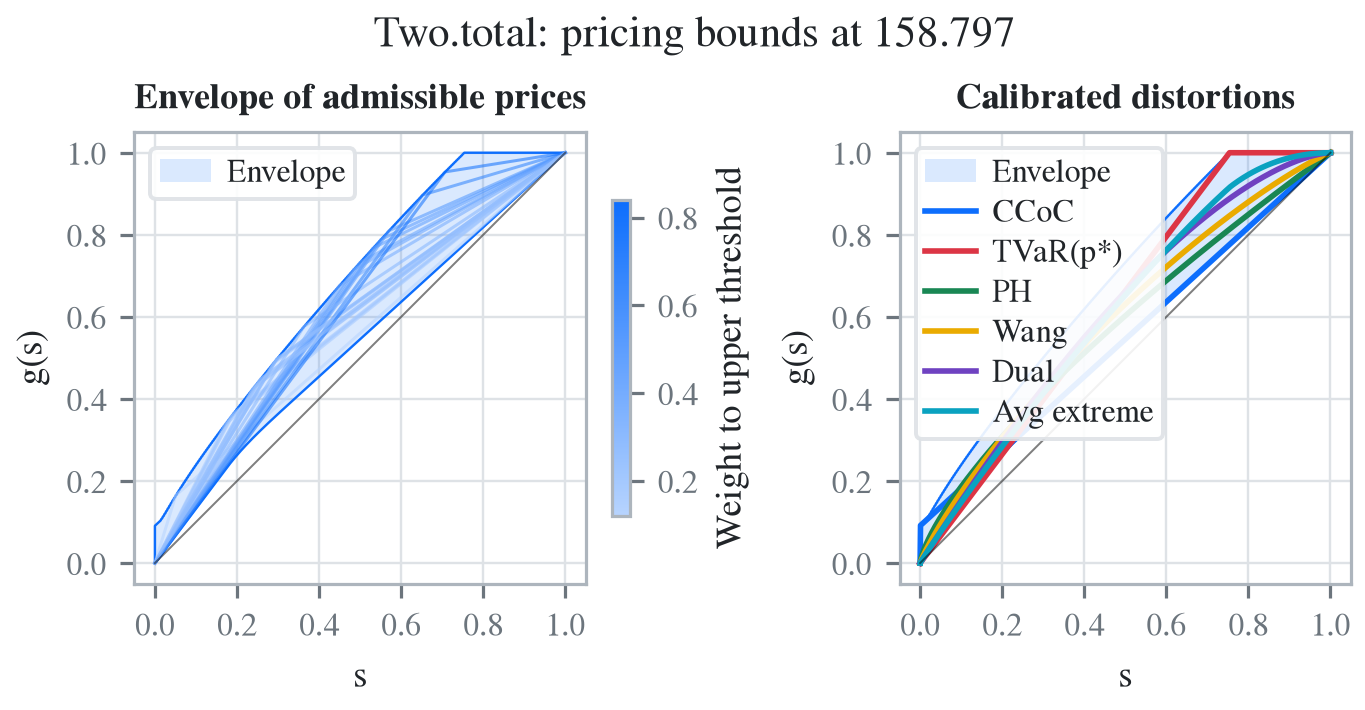

Bounds on the price of a layer

The envelope bounds the price of any other risk \(Y\) over \(G_P\), because \(g[Y] = \int g(S_Y(y))\,dy\) and \(g\) lies between the edges at every \(s\). For an aggregate layer \(l\) xs \(r\) on the total, \(S_Y(y) = S(r + y)\) for \(0 \le y < l\). The bounds hold but need not be sharp, because no one member of \(G_P\) attains an edge at every \(s\). The class PricingBounds computes the exact range, shown beside the envelope bounds for two layers, 50 xs 150 and 100 xs 250.

x, S, bs = port.density_df.loss, port.density_df.S, port.bs
lower = bd.cloud_df.min(axis=1).to_numpy()
layers, rows = {}, {}
for r, l in [(150, 50), (250, 100)]:
    name = f'{l} xs {r}'
    layers[name] = port.density_df.p_total.groupby(np.clip(x - r, 0, l)).sum()
    Sy = S.loc[r:r + l - bs].to_numpy()
    rows[name] = {'envelope lower': np.interp(Sy, bd.s_grid, lower).sum() * bs,
                  'envelope upper': bd.max_envelope(Sy).sum() * bs}
exact = PricingBounds(port, layers, a=a).bounds(P).droplevel('P')
GT(pd.DataFrame(rows).T.rename_axis('layer')
     .join(exact[['lower', 'upper']].add_prefix('exact ')), float_format='.3f')

layer	envelope lower	envelope upper	exact lower	exact upper
50 xs 150	13.792	19.770	14.098	18.497
100 xs 250	3.810	12.789	3.810	11.811

On 100 xs 250, \(S\) runs from 0.013 to 0.054, where the lower edge is the single distortion TVaR at \(p^*\), so the envelope lower bound, 3.810, is exact. The envelope upper bound, 12.789, is 0.98 above the exact 11.811. On 50 xs 150, \(S\) runs from 0.13 to 0.34, across the point where the lower edge changes distortion, and both envelope bounds are loose.

Refused inputs

A premium below the mean of \(X\) or above the assets is refused, and so is a unit that is not in the portfolio. The premium test uses the mean of \(X\), 138.667, and not \(L\).

refuse(lambda: Bounds(port, 130, a=a),
       lambda: Bounds(port, 400, a=a),
       lambda: Bounds(port, P, a=a, unit='Cat'))

premium 130.0 below mean 138.66655487886732; pricing bound undefined
premium 400.0 exceeds asset cap 365.125
unit 'Cat' not in portfolio 'Two'

Footnotes

1. All three from aggregate 1.0