Using AllocationBounds

Ranges of the natural allocation of a portfolio premium to each unit over all distortions that price the total

A distortion \(g\) that prices the total \(X\) of a portfolio to a premium \(P\) also allocates \(P\) to the units, by the natural allocation \[ A_i(g) = \sum_x \kappa_i(x)\,\bigl(g(S(x^-)) - g(S(x))\bigr), \qquad \kappa_i(x) = \mathsf{P}(X_i \mid X = x), \] where \(S\) is the survival function of \(X\), and the allocations add up to \(P\). Different distortions in the set \(G_P\) of those pricing \(X \wedge a\) to \(P\) allocate it differently. The class AllocationBounds¹ computes, for each unit, the range of \(A_i\) over \(G_P\).

In terms of the Kusuoka measure \(\mu\) of \(g\), \(A_i = \int a_i(p)\,\mu(dp)\), where \(a_i(p)\) is the natural allocation of \(\mathrm{TVaR}_p(X)\) to unit \(i\). The premium and the allocation are both linear in \(\mu\), so the extreme allocations are attained by biTVaRs, mixtures of two TVaRs, and the range of \(A_i\) is the vertical slice at \(\mathrm{TVaR}_X = P\) through the convex hull of the curve \(p \mapsto (\mathrm{TVaR}_p(X), a_i(p))\). On the discrete grid the curve is exactly piecewise linear with a vertex at each CDF breakpoint of \(X\), the pair of conditional tail expectations \((\mathsf{P}(X \mid X \ge x_m), \mathsf{P}(X_i \mid X \ge x_m))\), so the bounds are exact. With assets \(a\) the default states \(X \ge a\) collapse into one outcome at \(a\), which allocates \(a\,\mathsf{P}(X_i/X \mid X \ge a)\) to unit \(i\), the equal priority (linear) allocation.

The class AllocationBounds is a subclass of the same convex hull engine as PricingBounds (Using PricingBounds), which bounds the price of a risk on its own rather than its share of the portfolio premium. The class Bounds (Using Bounds) computes the envelope of the distortions in \(G_P\) themselves. Use AllocationBounds for the share of each unit. The hull is computed once, and the method bounds(P) slices it at any premium in premium_range. Because the allocations add up to \(P\), with two units the distortion that gives one unit its largest allocation gives the other its smallest, and the two ranges have the same width.

from aggregate.bounds import AllocationBounds
AllocationBounds(port, a=np.inf, units=None, s_floor=1e-14)
port.allocation_bounds(a=0, p=0, units=None)     # p sets a = port.q(p)

The portfolio must be updated, so that density_df contains the conditional expectations exeqa_<unit>. The argument units selects units, by default all of them. The method Portfolio.allocation_bounds with a and p both zero leaves the total uncapped.

import numpy as np
from aggregate import build, __version__
from aggregate.bounds import AllocationBounds
from style import wprint, GT, refuse, figures, figure
figures()
print(__version__)

2.1.0a5

Allocation ranges for two units

The example is the portfolio Two of Using Bounds. Unit Thin has 10 claims with a gamma severity of mean 10 and coefficient of variation (CV) 0.5, and unit Thick has 2 claims with a lognormal severity of mean 20 and CV 2, limited to 250. Assets are the 99th percentile of the total, \(a = 365.125\), and the premium \(P = 158.797\) earns a 10% cost of capital. The attribute info of AllocationBounds shows 5,843 vertices, feasible premiums from \(L = \mathsf{P}(X \wedge a) = 138.164\) to \(a\), and an additivity error of \(8.4 \times 10^{-9}\), the largest gap between TVaR and the sum of its unit allocations over the vertices.

port = build('''port Two
  agg Thin  10 claims sev gamma 10 cv 0.5 poisson
  agg Thick  2 claims 250 xs 0 sev lognorm 20 cv 2 poisson''')
a = port.q(0.99)
port.calibrate_distortions(0.10, a=a)
P = port.calibration_df.P.iloc[0]
ab = AllocationBounds(port, a=a)
wprint(ab.info)
GT(ab.bounds(P).droplevel('P'), float_format='.3f')

allocation bounds object Two
kind                     natural-allocation premium ranges by unit
asset cap                365.125
units                    Thin, Thick
vertices                 5843
premium range            [138.164, 365.125]
s_floor                  1e-14
additivity error         8.37e-09

unit	lower	upper	width
Thick	47.518	57.995	10.476
Thin	100.802	111.278	10.476

The allocation to Thick lies between 47.518 and 57.995, and to Thin between 100.802 and 111.278. Both ranges have width 10.476, and the lower end for Thin plus the upper end for Thick is \(P\). The width is 22% of the smallest allocation to Thick and 10% of the smallest to Thin.

Allocations under the five calibrated distortions

Each of the five calibrated distortions is in \(G_P\). The method port.price(a=a) computes its natural allocation of \(P\) (see Using price). The table lists the distortions in order of their Gini index, gini. Each allocation lies in the range, to within 0.001 at the ends: tvar gives Thick its smallest allocation and ccoc its largest, and here the allocation to Thick falls as gini rises.

alloc = port.price(a=a).df.P.unstack('unit').loc[port.distortion_df.index]
alloc.insert(0, 'gini', port.distortion_df.gini)
GT(alloc, float_format='.3f', formatters={'gini': '{x:.4f}'})

distortion	gini	Thick	Thin	total
ccoc	0.0909	57.995	100.801	158.797
ph	0.1556	53.978	104.819	158.797
wang	0.1868	51.814	106.983	158.797
dual	0.2196	49.511	109.286	158.797
tvar	0.2461	47.518	111.278	158.797

Distortions that attain the allocation bounds

The method bitvars(P) lists the biTVaR at each end of each range, as p0, p1, and the weight w1 on p1. The upper end for Thick and the lower end for Thin share one biTVaR, the mean mixed with TVaR at 0.99, which equals the maximum \(a\) of \(X \wedge a\), with weight \(0.0909\): the ccoc distortion. The other two ends share a bracket around \(p^* = 0.2461\), equivalent to TVaR at \(p^*\). The method distortion(P, unit, bound) returns the achieving Distortion. The method check(P) recomputes each allocation and the total premium from first principles with it. The largest errors are below \(10^{-12}\).

print(ab.check(P)[['err', 'total_err']].abs().max().to_dict())
GT(ab.bitvars(P).droplevel('P'), float_format='.4f')

{'err': 1.5631940186722204e-13, 'total_err': 6.252776074688882e-13}

unit	bound	value	p0	p1	w1
Thick	lower	47.5185	0.2457	0.2462	0.9083
	upper	57.9950	0.0000	0.9900	0.0909
Thin	lower	100.8020	0.0000	0.9900	0.0909
	upper	111.2785	0.2457	0.2462	0.9083

The allocation curves

The table curve_df lists the vertices, indexed by \(p\), with \(\mathrm{TVaR}_p(X \wedge a)\) in exeqa_total and \(a_i(p)\) in exeqa_<unit>. The first row, \(p = 0\), contains the expected losses by unit, 99.859 and 38.306, which add up to \(L\). The last is the default outcome at \(a\), which allocates 110.237 to Thin and 254.888 to Thick.

GT(ab.curve_df.iloc[[0, -1]], float_format='.3f')

p	exeqa_total	exeqa_Thin	exeqa_Thick
0.000	138.164	99.859	38.306
0.990	365.125	110.237	254.888

The plot shows the curve of each unit, its lower and upper hulls, and the slice at \(P\). The curve for Thin rises and then falls: far in the tail the total is large mainly because Thick is large, so the allocation of TVaR to Thin shrinks. The lower hull of Thin and the upper hull of Thick are both the chord from the first vertex to the last, whose points are the ccoc distortions at different costs of capital.

fig, axs = figure('full', cols=2)
ab.plot(P=P, axs=axs);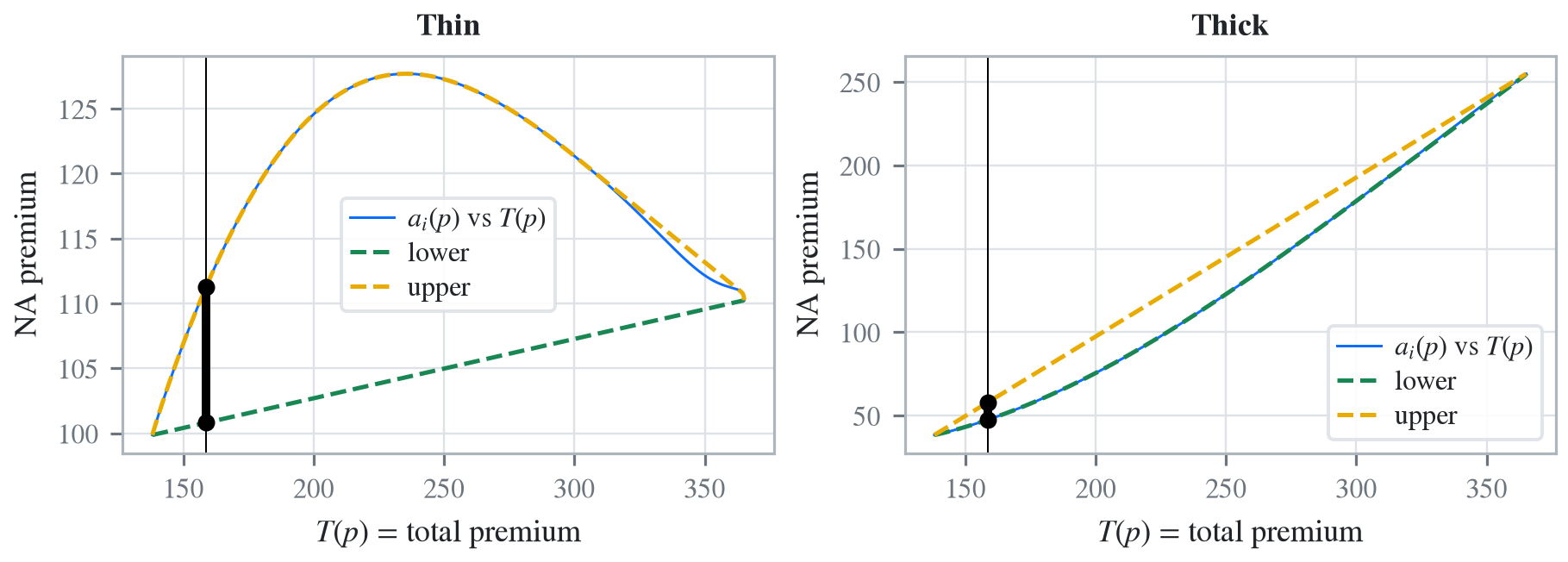

Refused inputs

A unit that is not in the portfolio is refused, and so is a premium outside premium_range.

refuse(lambda: AllocationBounds(port, a=a, units=['Cat']),
       lambda: ab.bounds(130))

density_df missing columns ['exeqa_Cat']; check unit names ['Cat'].
P=[130.] outside feasible premium range [138.164, 365.125] (= [E[X], TVaR at
s_floor truncation]).

Footnotes

1. From aggregate 1.0