Using occurrence reinsurance

Per-occurrence excess of loss layers, partial placements and towers (occurrence net of, occurrence ceded to)

An occurrence layer y xs a placed at share \(s\) pays \(s\min((x - a)^+, y)\) on a claim of size \(x\). A program of non-overlapping layers pays the sum, \(c(x) = \sum_j s_j \min((x - a_j)^+, y_j)\), and the cedant keeps \(n(x) = x - c(x)\). Over a year with claims \(X_1, \dots, X_N\) the ceded loss is \(C = \sum_i c(X_i)\) and the net loss is \(\sum_i n(X_i)\), and the two add to the gross loss. Each view is an ordinary compound distribution, with the same claim count and the severity transformed by \(c\) or \(n\), so aggregate computes it by the same convolution as the gross.

The clause occurrence net of makes the aggregate the net view and occurrence ceded to makes it the ceded view. The clause follows the severity and precedes the frequency, and every layer is written bottom up. A partial placement is written with po (part of): a percentage is the share, and a bare number is an amount, so 250 po 500 xs 500 is a 50% share. Layers are joined by and, and tower followed by a list of breakpoints is shorthand for the consecutive full layers between them. A layer can be named with as, and the name is used by the structure chart and by a P&L walk. The annual terms aad and agglimit are described in Using aad and agglimit.

occurrence net of 250 xs 250
occurrence net of 50% po 500 xs 500           # 50% share
occurrence net of 250 po 500 xs 500           # the same: 250 of 500
occurrence ceded to 250 xs 250 and 50% po 500 xs 500 as "Middle"
occurrence ceded to tower [250 500 1000 2000] # 250 xs 250, 500 xs 500, 1000 xs 1000

from aggregate import build, qd, __version__
from style import wprint, GT, refuse, figures
figures()
print(__version__)

1.60.0

Net and ceded views of one program

The example book has 20 claims a year from a lognormal severity with mean 100 and coefficient of variation (CV) 3, limited to 2,000. It cedes a program of three layers: 250 xs 250 in full, then 500 xs 500 and 1,000 xs 1,000, each half placed. Written occurrence net of, the aggregate is the net loss, and qd shows the net severity and the net annual loss.

book = '''agg {} 20 claims 2000 xs 0 sev lognorm 100 cv 3
  occurrence {}
    250 xs 250 and 50% po 500 xs 500 and 500 po 1000 xs 1000
  poisson'''
net = build(book.format('Net', 'net of'))
qd(net)

Aggregate object: Net. Frequency distribution poisson. Severity lognorm,
[0, 2,000], bounded; 2,000 xs 0. Updated with bucket size 1/2 and log2 =
16. Validation: reinsurance; subject not unreasonable; net not
unreasonable.

       Mean     SD      CV    Skew P01 Median    P99
X                                                   
Freq     20 4.4721 0.22361 0.22361                  
Sev  73.469 111.58  1.5188  3.9118   1   31.5  539.5
Agg  1469.4 597.48 0.40662 0.80416 428 1387.5 3199.5

Written occurrence ceded to, the same program gives the ceded loss. Both aggregates compute all three views, and reins_explanation gives the split of the gross expected loss: 1,901.37 gross, 432.00 ceded, and 1,469.38 net. The ceded mean is the mean of the ceded to aggregate.

ceded = build(book.format('Ceded', 'ceded to'))
wprint(net.reins_explanation)
print(f'{ceded.est_m:.2f}')

Net of 100% share of 250 xs 250 and 50% share of 500 xs 500 and 50% share of
1,000 xs 1,000 per occurrence. Per occurrence, gross expected loss 1,901.37
splits into 431.997 ceded (22.7%) and 1,469.38 net.
432.00

The method reins_occ_plot draws the three views per claim on the left, as densities on a log scale, and for the year on the right, as quantile functions (a Lee diagram). The net claim has an atom at 250, the retention of the full first layer.

fig = net.reins_occ_plot()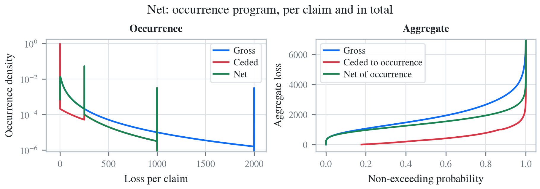

Partial placements and towers

The property reins_description shows each layer as a share of a limit in excess of an attachment. A percentage and an amount give the same share, and a tower expands to full layers between consecutive breakpoints, starting from the first. The descriptions are available before the aggregate is updated.

stub = 'agg T 20 claims 2000 xs 0 sev lognorm 100 cv 3 occurrence ceded to {} poisson'
for layer in ['50% po 500 xs 500', '250 po 500 xs 500', 'tower [250 500 1000 2000]']:
    wprint(f'{layer:26s}', build(stub.format(layer), update=False).reins_description)

50% po 500 xs 500          Ceded to 50% share of 500 xs 500 per occurrence
250 po 500 xs 500          Ceded to 50% share of 500 xs 500 per occurrence
tower [250 500 1000 2000]  Ceded to 100% share of 250 xs 250 and 100% share of
                           500 xs 500 and 100% share of 1,000 xs 1,000 per
                           occurrence

A gap between layers can be left as a hole, as in 250 xs 250 and 1000 xs 1000, or written as a layer with zero share, 0% po 500 xs 500. A bare amount below 5% of the limit, such as 0.5 po 500 xs 500, gives a placement of 0.1% and logs a warning suggesting the percentage form.

Reinsurance statistics by layer

The table reins_stats_df has one column per layer, layer.1 to layer.3, beside Gross and the program totals Ceded and Net. The meta rows give the terms and the probabilities: pr_attach is the probability that a claim exceeds the attachment, pr_detach the probability that it exhausts the layer, and lol (loss on line) the expected annual layer loss over the placed limit. The freq, sev, and agg rows give the moments. The table below shows the main rows, transposed so that each column of the original is a row.

rows = [('meta', 'share'), ('meta', 'limit'), ('meta', 'attach'),
        ('meta', 'pr_attach'), ('meta', 'pr_detach'), ('meta', 'lol'),
        ('freq', 'mean'), ('sev', 'mean'), ('agg', 'mean'), ('agg', 'cv')]
s = net.reins_stats_df.droplevel('view', axis=1).loc[rows].T
s.columns = [m if c == 'meta' else f'{c} {m}' for c, m in s.columns]
GT(s, float_format=',.4g')

layer	share	limit	attach	pr_attach	pr_detach	lol	freq mean	sev mean	agg mean	agg cv
Gross	1	2,000	0	0.9993	0.003139	0.9507	20	95.07	1,901	0.5296
layer.1	1	250	250	0.08641	0.03445	1.088	1.728	157.5	272.1	0.8825
layer.2	0.5	500	500	0.0344	0.01142	0.3975	0.6881	144.4	99.39	1.435
layer.3	0.5	1,000	1,000	0.01141	0.003139	0.121	0.2283	265.1	60.51	2.552
Ceded	—	1,000	250	0.08641	—	0.432	20	21.6	432	1.066
Net	—	—	—	0.9993	—	—	20	73.47	1,469	0.4066

A layer column is conditional on a claim reaching the layer. The first layer is reached by \(20 \times 0.08641 = 1.728\) claims a year, whose mean payment is 157.5, for an expected annual loss of 272.1. The second layer’s loss on line is \(99.39/(0.5 \times 500) = 0.398\), on the placed limit. The Ceded and Net columns are unconditional, with the gross claim count, and their severity means, 21.60 and 73.47, add to the gross 95.07. The limit of Ceded, 1,000, is the placed capacity \(250 + 0.5 \times 500 + 0.5 \times 1000\).

st = net.reins_stats_df['occ']
print(f"{20 * st.loc[('meta', 'pr_attach'), 'layer.1']:.4f}",
      f"{st.loc[('freq', 'mean'), 'layer.1'] * st.loc[('sev', 'mean'), 'layer.1']:.2f}")
print(f"{st.loc[('sev', 'mean'), 'Ceded'] + st.loc[('sev', 'mean'), 'Net']:.4f}",
      f"{st.loc[('sev', 'mean'), 'Gross']:.4f}")

1.7281 272.10
95.0687 95.0687

The table reins_summary_df compares each view with the gross by component, and reins_density_df contains the gross, ceded, and net severities and aggregates on the grid, one column each. The joint law of ceded and net is a bivariate distribution, the subject of Using grossnet, grossceded and netceded.

Aggregate covers and pricing clauses

The same layer clauses after the frequency, as aggregate net of or aggregate ceded to, apply to the annual loss rather than to each claim. An occurrence program inures to an aggregate cover, so the aggregate layers apply to the output of the occurrence stage.

A layer also accepts a premium, deposit, rol (rate on line), or rate (a fraction of subject premium), and a ceding commission cede. They describe the economics of the cession, which only a profit and loss statement can book. A plain agg builds the loss structure, drops the pricing clauses with an IgnoredDecLClauseWarning, and keeps them in its stored program, so that a pnl or xpnl referring to it books them: see Using pnl and xpnl.

Refused programs

Layers must be entered bottom up and must not overlap, and a share cannot exceed 100%, whether it comes from a percentage or from an amount above the limit. Occurrence reinsurance acts on each claim, so it cannot be combined with approximate, which replaces the aggregate by a fitted distribution.

pre = 'agg R 20 claims 2000 xs 0 sev lognorm 100 cv 3 occurrence net of '
refuse(pre + '500 xs 500 and 250 xs 250 poisson',
       pre + '500 xs 250 and 500 xs 500 poisson',
       pre + '150% po 500 xs 500 poisson',
       pre + '600 po 500 xs 500 poisson',
       pre + '250 xs 250 poisson approximate gamma')

Reinsurance layers must be entered bottom-up (lowest attachment first); got
attachment 250.0 after 500.0. Enter layers in ascending order and use "0 po L xs
A" to represent a gap.
Reinsurance layers overlap: layer attaching at 500.0 starts below the top
(750.0) of the preceding layer. Layers must be non-overlapping; use "0 po L xs
A" to represent a gap.
share 1.5 on '500 xs 500' exceeds 100%; a bare number before po is an amount of
the limit, a percentage is the share
share 1.2 on '500 xs 500' exceeds 100%; a bare number before po is an amount of
the limit, a percentage is the share
DecL: approximate is incompatible with occurrence reinsurance (the
method-of-moments fit bypasses the per-occurrence convolution); use aggregate
reinsurance instead.