Using the structure chart

Reinsurance program diagrams of layers, shares and retentions, with optional Lee curves (the structure chart)

The structure chart draws a reinsurance program the way a broker’s slide does. A gross block on the left shows the subject book. Beside it, each cession stage is a tower over its loss axis: one for the occurrence program, with loss per claim, and one for the aggregate program, with annual loss. Each placed layer is a rectangle from its attachment to its exhaustion point, and its width is its share. The unplaced part of a layer is hatched (co-participation), retentions are gray, and an uncovered band is drawn as a gap with a cross hatch. The loss axis of a tower is ticked at its layer boundaries rather than on a continuous scale.

Each block is annotated with fields selected by the annotate argument from geometry, premium, el (expected loss), lr (loss ratio), rol (rate on line), lol (loss on line), sd, pr_attach, pr_detach, reinstatements, and cede, always in that order. The default is ('geometry', 'premium', 'el', 'lr'). A field is available at one of three tiers, and a field whose tier is not reached is omitted, so one selection works on any object.

1. Declared: the terms and name of each layer, available before the aggregate is updated.
2. Built: the risk statistics from reins_stats_df (el, sd, lol, pr_attach, pr_detach), on an updated aggregate.
3. Priced: premium, lr, rol, cede, and reinstatements, on a pnl or xpnl only, because a plain agg drops pricing clauses (see Using pnl and xpnl).

Premium, expected loss, and standard deviation are annual and shown at 100% terms, as a layer is quoted. With lee=True, the chart of an updated object also shows, beside each tower and on the same loss axis, the quantile function (Lee curve) of the distribution that tower is read against: the gross claim severity for the occurrence tower, and for the aggregate tower the annual loss after the occurrence program, which is the subject of the aggregate cover. Faint lines extend each boundary across to the curve.

The function build_chart_doc returns the chart as a ChartDoc, which contains the blocks and curves as data. The function plot_chartdoc draws it with matplotlib. The module aggregate.charts is provisional: its interface may change in a minor release.

doc = build_chart_doc(obj, 'structure', annotate=..., lee=False)  # obj: Aggregate or PnL
fig = plot_chartdoc(doc, return_period=False, log=False)

import numpy as np
from aggregate import build, __version__
from aggregate.charts import available_charts, build_chart_doc
from aggregate.plots import plot_chartdoc
from style import wprint, refuse, figures
figures()
print(__version__)

1.54.0

The declared and built tiers on an aggregate

The example book has 20 claims a year from a lognormal severity with mean 100 and coefficient of variation 3, limited to 2,000, and an occurrence program of three named layers: Working, 250 xs 250 in full, Middle, 90% of 500 xs 500, and Top, 75% of 1,000 xs 1,000. The structure chart is available as soon as the program is declared. The function available_charts lists it with the other charts of the object.

book = '''agg Book 20 claims 2000 xs 0 sev lognorm 100 cv 3
  occurrence net of
    250 xs 250 as "Working" and
    90% po 500 xs 500 as "Middle" and
    75% po 1000 xs 1000 as "Top"
  poisson'''
u, a = build(book, update=False), build(book)
print(available_charts(u))

['structure', 'reins']

The same selection of fields gives only the terms on the declared object and adds the statistics on the built one. The tiers reached are recorded in the document’s meta. The expected loss of Middle is 198.8 at 100%, so the expected loss of the 90% placed share is \(0.9 \times 198.8 = 178.9\), the mean of layer.2 in reins_stats_df. Loss on line is the same on either basis.

fields = ('geometry', 'el', 'sd', 'lol', 'pr_attach', 'pr_detach')
for obj in [u, a]:
    doc = build_chart_doc(obj, 'structure', annotate=fields)
    print(doc.meta['tiers'])
    for b in doc.blocks:
        if b.role == 'layer':
            wprint(f'  {b.label:8s}', ', '.join(b.label_lines))
print(f"{a.reins_stats_df.loc[('agg', 'mean'), ('occ', 'layer.2')]:.1f}")

['declared']
  Working  250 xs 250
  Middle   90.0% po 500 xs 500
  Top      75.0% po 1,000 xs 1,000
['declared', 'built']
  Working  250 xs 250, el 272.1, lol 108.8%, sd 240.1, pr attach 8.6%, pr detach
           3.4%
  Middle   90.0% po 500 xs 500, el 198.8, lol 39.8%, sd 285.1, pr attach 3.4%,
           pr detach 1.1%
  Top      75.0% po 1,000 xs 1,000, el 121, lol 12.1%, sd 308.8, pr attach 1.1%,
           pr detach 0.3%
178.9

Lee curves and return periods

With lee=True each tower is joined to its Lee curve. Drawn with return_period=True and a log scale on the horizontal axis, the curve gives the return period of every boundary. The renderer drops any annotation line that does not fit inside its block: the partial layers Middle and Top are too narrow for their terms, and the short Working block has no room for its expected loss.

fig = plot_chartdoc(build_chart_doc(a, 'structure', lee=True),
                    return_period=True, log='x')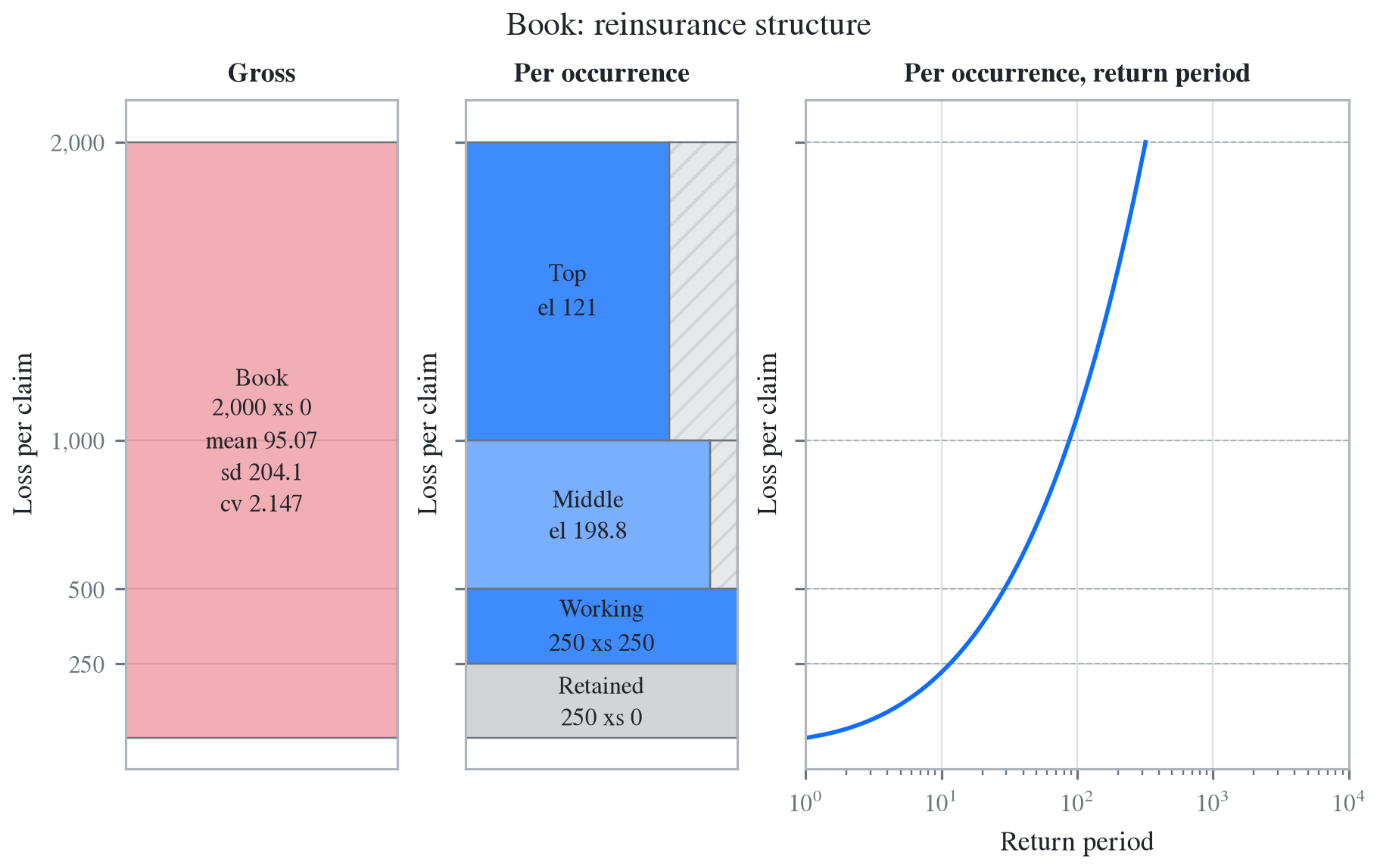

On the occurrence tower the curve is the quantile function of the claim severity, so its return period counts claims, not years. The attachment of Working is exceeded by one claim in 11.6, and with 20 claims a year it is exceeded in 82% of years, an annual return period of 1.2 years. The annual figures assume a Poisson count, and the conversion is described in Using oep. The aggregate tower’s curve is an annual distribution, and its return period is in years.

for x in [250, 500, 1000]:
    s = a.sev.sf(x)
    annual = -np.expm1(-a.n * s)
    print(f'{x:5d}  {1 / s:5.1f} claims  {annual:.4f}  {1 / annual:4.2f} years')

  250   11.6 claims  0.8228  1.22 years
  500   29.0 claims  0.4977  2.01 years
 1000   87.6 claims  0.2042  4.90 years

The priced tier on an xpnl

The xpnl below wraps the example book with a premium on each layer and adds an aggregate stop loss, 1,000 xs 2,000, on the annual net of the occurrence program. Every field is now available. Premium is shown at 100% terms: the Middle layer is rated at 55% on line, a premium of 275 for the full layer, and its loss ratio is \(198.8/275 = 72.3\%\). The placed premiums, 375, 247.5, and 135, are listed in the economics of the PnL. The aggregate tower is read against the annual net loss, so its statistics are annual.

x = build('''xpnl BookX 2500 premium less
  agg BookX 20 claims 2000 xs 0 sev lognorm 100 cv 3
    occurrence net of
      250 xs 250 rol 150% as "Working" and
      90% po 500 xs 500 rol 55% cede 10% as "Middle" and
      75% po 1000 xs 1000 rol 18% as "Top"
    poisson
    aggregate net of 1000 xs 2000 rol 4% as "Stop loss"''')
doc = build_chart_doc(x, 'structure',
                      annotate=('geometry', 'premium', 'el', 'lr', 'rol', 'cede'))
print(doc.meta['tiers'], [round(v, 2) for v in x.economics['pc_occ_by_layer']])
fig = plot_chartdoc(doc)

['declared', 'built', 'priced'] [375.0, 247.5, 135.0]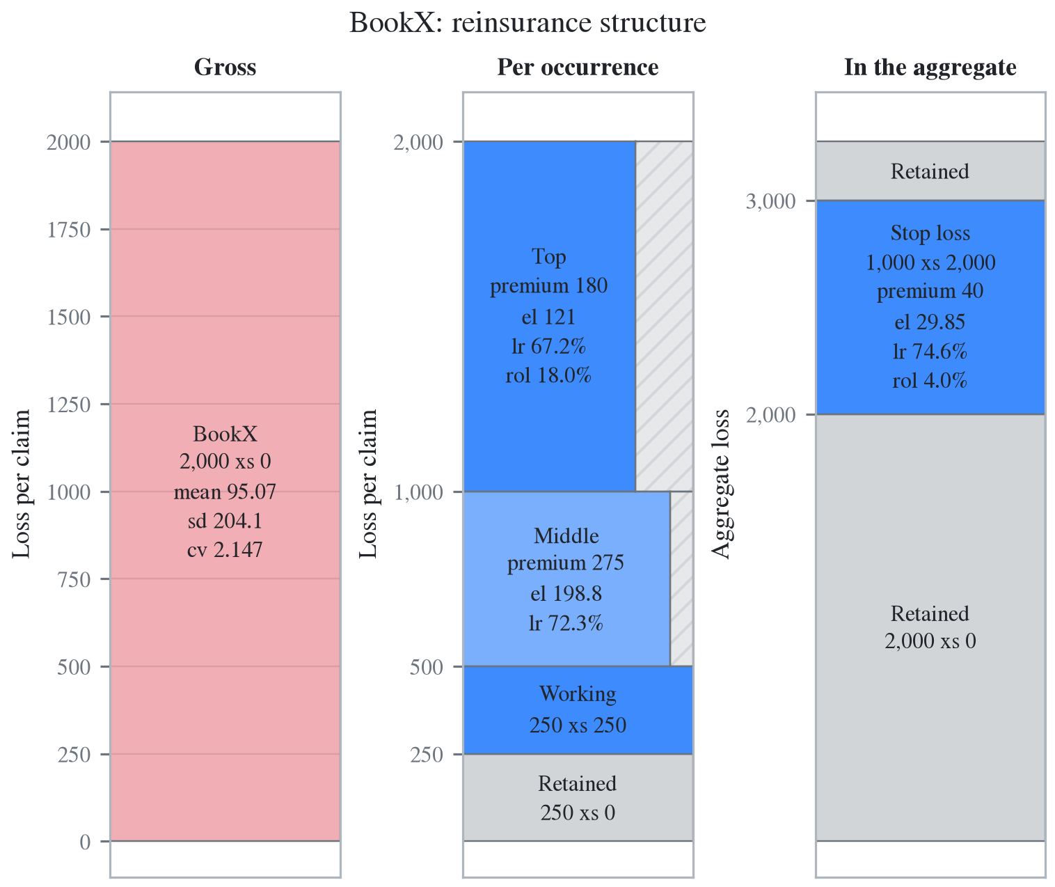

The Middle block shows three of its six annotation lines, losing its terms for width and its rate on line and commission for height. The full annotation of every layer is in the document.

for b in doc.blocks:
    if b.role == 'layer':
        wprint(f'{b.label:9s}', ', '.join(b.label_lines))

Working   250 xs 250, premium 375, el 272.1, lr 72.6%, rol 150.0%
Middle    90.0% po 500 xs 500, premium 275, el 198.8, lr 72.3%, rol 55.0%, cede
          10.0%
Top       75.0% po 1,000 xs 1,000, premium 180, el 121, lr 67.2%, rol 18.0%
Stop loss 1,000 xs 2,000, premium 40, el 29.85, lr 74.6%, rol 4.0%

Refused requests

A Lee curve needs an updated object, an annotate field must be one of those listed in the error message, and an aggregate with no reinsurance has no structure chart. Each request raises a ValueError.

plain = build('agg Plain 20 claims 2000 xs 0 sev lognorm 100 cv 3 poisson')
refuse(lambda: build_chart_doc(u, 'structure', lee=True),
       lambda: build_chart_doc(a, 'structure', annotate=('el', 'var')),
       lambda: build_chart_doc(plain, 'structure'))

chart_structure: lee=True needs the realized grid: call Book.update() first, or
take the geometry-only chart the default gives.
unknown annotate field(s) ['var']; expected a subset of ('geometry', 'premium',
'el', 'lr', 'rol', 'lol', 'sd', 'pr_attach', 'pr_detach', 'reinstatements',
'cede')
chart 'structure' is not available for Aggregate 'Plain': its availability
predicate failed (missing update() grid, or required structure such as
reinsurance)