Using AggregateCHF with stable laws

Accurate stable distributions by tilted inversion, checked against scipy

A stable law with index \(\alpha < 2\) has a power tail, \(\Pr(X > x) \sim A x^{-\alpha}\), and no severity to discretize: it is the limit of a Pareto book as the claim count grows (Using stable). Its characteristic function is in closed form, so the class AggregateCHF (Using AggregateCHF) computes it on a grid, accurately into the far tail¹. In comparison, scipy.stats.levy_stable is slow in the body of the distribution and wrong past a few hundred scales. A chfagg takes the parameters of a stable law but not a reference such as stable.x (Using stable names and arithmetic).

The difficulty is aliasing. Inverting on a window of length \(W\) folds the mass beyond it back in, and a power tail has a great deal of mass beyond any window: holding the wrapped mass to \(10^{-6}\) untilted takes \(2^{23}\) buckets at \(\alpha = 1.1\) and \(2^{34}\) at \(\alpha = 0.7\). Worse, the mass from \(x + W\) lands on \(x\), so near the right edge the relative error is of order one whatever the total. The cure is to invert along a shifted contour. For \(\beta = 1\) the left tail is light and \(\varphi\) is analytic on the upper half plane, so the line of integration moves to \(\mathrm{Im}\,s = \theta\): \[ e^{-\theta x_k}p_k = \frac{1}{2\pi}\int \varphi(t + i\theta)\,h\,\mathrm{sinc}\big((t+i\theta)h/2\big)\,e^{-itx_k}\,dt . \] What wraps is the damped sequence \(e^{-\theta x}p\), and multiplying back by \(e^{\theta x_k}\) recovers the masses. Written as \(\tau = \theta W\) e-folds across the window, the wrap costs \(\rho e^{-\tau}\) and the amplified roundoff \(\varepsilon\kappa e^{\tau}\), both relative to the mass at the right edge; the engine takes the \(\tau^*\) that balances them and reports the balance as edge_error. Tilting halves the number of digits the window’s dynamic range costs. The mass beyond the window is no longer folded in: it is left out and reported as outside_above, so sf stays right across the window and the first bucket holds whatever lies below it.

import warnings
import numpy as np
import scipy.stats as ss
from aggregate import build, qd, __version__
from aggregate.characteristic_function import AggregateCHF
from aggregate.constants import ValidationWarning
from aggregate.stable import Stable
from style import wprint, GT, figures, figure
figures()
# some of these laws fail their verdicts on purpose, and the text discusses each
warnings.simplefilter('ignore', ValidationWarning)
print(__version__)

1.58.0

chfagg S 2 * stable 1.5 1 + 10            # alpha beta [s0|s1], scaled and shifted, tilted
chfagg W stable 0.7 1 hints{tilt=False}   # untilted, wrapping, for teaching
chfagg T stable 1.5 0.5                   # two heavy tails: split, each half tilted

A totally skewed stable law on a tilted grid

The law stable 1.5 1 at unit scale is the limit law of a Pareto book with tail index 1.5. The DecL statement chfagg S stable 1.5 1² declares it, and build returns it updated. The attribute info reports the tilt pair (left, right) in e-folds, \(\theta\) per unit of loss, the mass left outside the window, and the modeled edge error. The window reaches about 2,000 at log2 16, with a bucket of 1/32.

s = build('chfagg S stable 1.5 1')
wprint(s.info)

aggregate object name    S
value_type               loss
claim count              n/a
frequency distribution   n/a
severity distribution    n/a
loss table               n/a
approximate              exact
bs                       1/32
log2                     16
padding                  n/a
sev_calc                 n/a
dsev_bucket              n/a
normalize                False
x_min                    -10.7812
x_max                    2,037.19
premium                  n/a
expected loss            -0.0265159
loss ratio               n/a
P(X=0)                   0.00617238
validation_eps           0.0001
reinsurance              none
occurrence reinsurance   no reinsurance
aggregate reinsurance    no reinsurance
validation               not unreasonable
family                   stable
parameters               stable 1.5 1
support                  -inf to inf
scale                    1
total mass               0.999996
outside mass             4.34e-06, below 0, above 4.34e-06
tilt                     (0, 8.32)
theta                    (0, 0.00406)
edge error               0.000164
truncation error         0
transfer sigma           n/a
most negative bucket     2.42e-14
buckets per scale        32
checks                   7 ok
frequency tail           none: a characteristic function law
severity tail            none: a characteristic function law
aggregate tail           (-inf, inf), left super-exponential, right power-law
                         [power-law, alpha=1.5, infinite variance]
bounded                  False
id                       F5834EE7

In the body the grid agrees with scipy to six figures; the grid’s sf(x) is the law’s survival at \(x + h/2\), the bucket’s upper edge. At 1,000 scipy already returns zero, the tail constant \(A x^{-1.5}\) is the reference, and the grid matches it to \(4\times10^{-5}\). Beyond the window, which ends near 2,000, the grid reports the mass it leaves out as outside_above rather than a number it does not have.

u = Stable(1.5, 1)
h = s.bs
for x in [10, 100, 1000]:
    print(f'{x:6d} {s.sf(x):12.5e} {u.sf(x + h / 2):12.5e} {u.tail_constant * (x + h / 2) ** -1.5:12.5e}')
print(f'{u.sf(5430):.3g}', f'{s.outside_above:.3e}', f'{s.x_max:,.0f}')

    10  1.25322e-02  1.25322e-02  1.25862e-02
   100  3.98847e-04  3.98847e-04  3.98849e-04
  1000  1.26149e-05  0.00000e+00  1.26154e-05
0 4.339e-06 2,037

A totally skewed stable law without tilting

The hint hints{tilt=False}, or the call update(tilt=False), inverts the law on the real line and lets it wrap, for comparison with the tilted grid. The window is sized to hold the mass budget on both sides and has the same length as the tilted window, but the modeled error at its right edge is 0.32, compared with \(1.6\times10^{-4}\) on the tilted grid. Against the tilted answer, the untilted survival is two parts in a thousand low at 100 and a quarter low at 1,000.

w = build('chfagg W stable 1.5 1 hints{tilt=False}')
print(w.tilt, f'{w.edge_error:.2f}', f'{s.edge_error:.1e}')
for x in [100, 1000]:
    print(f'{x:6d} {w.sf(x):12.5e} {s.sf(x):12.5e}')

(0.0, 0.0) 0.32 1.6e-04
   100  3.97998e-04  3.98847e-04
  1000  9.35487e-06  1.26149e-05

A number given as the argument tilt is the tilt in e-folds: tilt=8 damps the wrap by \(e^{-8}\) and amplifies roundoff by \(e^{8}\). The automatic choice sits near 8 here, so the two grids are close.

w.update(tilt=8)
print(w.tilt, s.tilt, f'{np.abs(w.agg_density - s.agg_density).max():.1e}')

(0.0, 8.0) (0.0, 8.323062028545595) 9.2e-15

Coverage, the bucket cap, and the recommended grid

Because the tilt amplifies the truncation error too, the bucket is capped at \(\min(\gamma/10,\ \pi\gamma/(52\log 2)^{1/\alpha})\), and a small \(\alpha\) makes the cap bind: at \(\alpha = 0.7\) it is 1/64, the window is \(1{,}024\) scales long at log2 16, and half a percent of the law lies beyond it. The grid is accurate where it reaches, to \(10^{-6}\) in the body, and the checks line of info flags the coverage. Where a larger grid would cover the budget that line gives it as a paste-ready hints{} clause; here none up to log2 24 does, since the budget of \(10^{-5}\) needs a window of \(10^7\) scales, and the line reports that. The verdict is grid infeasible for this law, with the deficit. The method sharpen moves toward the recommended grid one log2 per call, confirming a grid once its outside mass is within the budget.

t = build('chfagg T stable 0.7 1')
wprint(t.validation_description)
print('\n'.join(ln for ln in t.info.splitlines() if ln.startswith(('total mass', 'outside mass', 'edge error', 'tilt', 'checks'))))
print(t.recommended_grid())

grid infeasible for this law; fails pmf deficit 5.792e-03
total mass               0.994208
outside mass             0.00579, below 0, above 0.00579
tilt                     (0, 12.3)
edge error               9.83e-06
checks                   6 ok, 1 flag: outside mass, coverage needs log2 above 24; log2=24 with bs=0.015625 is the most this engine offers
(24, 0.015625)

At \(\alpha = 1/2\) and \(\beta = 1\) the stable law is the Lévy law, which scipy has in closed form, so every bucket can be checked. The masses agree to \(10^{-6}\) relative across the body and the outside mass equals the exact survival at the window’s end.

l = AggregateCHF('L', 'stable', alpha=0.5, beta=1)
l.update()
lv = ss.levy()
exact = lv.cdf(l.xs + l.bs / 2) - lv.cdf(l.xs - l.bs / 2)
body = exact > 1e-6
print(f'{(np.abs(l.agg_density - exact)[body] / exact[body]).max():.1e}',
      f'{l.outside_above:.6f}', f'{lv.sf(l.x_max + l.bs / 2):.6f}')

2.5e-07 0.070432 0.070432

A law with a mean and a power tail has a window mean short of the theoretical mean by the tail beyond the window, at any grid size. The verdict therefore reads the completed mean, the window mean plus that tail in closed form, which recovers the theoretical mean: 2 * stable 1.5 1 + 10 has the verdict not unreasonable. The attribute validation_explanation gives both means. The method sharpen leaves the mean out of its score, since no grid under the bucket cap closes the gap in the window mean.

c = build('chfagg S 2 * stable 1.5 1 + 10')
print(c.validation_description)
wprint(next(s for s in c.validation_explanation.split('. ') if 'completed mean' in s))
wprint(c.sharpen().sharpen_description)

not unreasonable
The law has a power tail, so the window mean 9.94692 omits the tail beyond it,
0.0530761 in closed form; the completed mean 10 against the theoretical 10 is
the check the window cannot make
Sharpen: not run, the grid already scores 0.28 against a target of 0.5 and its
outside mass is within the budget.

Stable laws skewed to the left and the first bucket

A law with \(\beta = -1\) is the negative of one with \(\beta = 1\), and is computed that way: the tilt damps its heavy left tail, the window runs from far below to a few scales above the location, and the mass below the window is added to the first bucket, so cdf is right across the window. The first bucket means “the left edge and everything below it”.

m = AggregateCHF('M', 'stable', alpha=1.5, beta=-1)
m.update()
print(m.tilt, f'{m.x_min:,.0f}', f'{m.x_max:,.2f}', f'{m.outside_below:.2e}')
print(f'{m.agg_density[0]:.2e}', f'{m.cdf(-1000):.5e}', f'{s.sf(1000 - h):.5e}')

(8.323062028545595, 0.0) -2,037 10.78 4.34e-06
4.34e-06 1.26162e-05 1.26155e-05

Stable laws with two heavy tails

A law with \(|\beta| < 1\) has a power tail on each side, and no single contour serves it: \(\mathsf{P}e^{\theta X}\) is infinite for every \(\theta \ne 0\). The S1 law splits exactly instead, \(X = X_+ + X_-\) with \(X_+ \sim S(\alpha, 1, \gamma_+, \delta_1)\) and \(X_- \sim S(\alpha, -1, \gamma_-, 0)\), \(\gamma_\pm = \gamma\,((1 \pm \beta)/2)^{1/\alpha}\). Each half has one heavy tail, is tilted toward its light side on twice the grid, and the two are combined by a linear convolution so that nothing wraps; the window kept is the one leaving equal mass below and above, so its left edge is an output rather than an input. tilt reports the pair \((\tau_-, \tau_+)\) and outside_below and outside_above the balanced masses. Near \(|\beta| = 1\) the light half is narrower than a bucket and a normal law is moved from the wide half to the narrow one to resolve it, which transfer_sigma reports.

two = AggregateCHF('Two', 'stable', alpha=1.5, beta=0.5)
two.update()
print(two.tilt, f'{two.x_min:,.0f}', f'{two.x_max:,.0f}', f'{two.outside_below:.2e}', f'{two.outside_above:.2e}')
near = AggregateCHF('Near', 'stable', alpha=1.5, beta=0.99)
near.update()
print(near.tilt, f'{near.transfer_sigma / near.bs:.1f}', f'{near.edge_error:.1e}')

(5.432747148712065, 6.3485194215615826) -1,330 2,766 2.06e-06 2.06e-06
(3.021108943934432, 7.45121996689686) 2.5 2.2e-04

Both tails agree with scipy at 50 scales, to six figures, and both are still there at 500, where scipy returns zero on either side. The left tail of stable 1.5 0.5 has a constant equal to a third of the right tail’s constant, \((1-\beta)/(1+\beta)\).

v = Stable(1.5, 0.5)
for x in [-500, -50, 50, 500]:
    ref = v.cdf(x + two.bs / 2) if x < 0 else v.sf(x + two.bs / 2)
    got = two.cdf(x) if x < 0 else two.sf(x)
    print(f'{x:6d} {got:12.5e} {ref:12.5e}')
print(f'{v.left_tail_constant / v.tail_constant:.3f}')

  -500  8.92370e-06  0.00000e+00
   -50  2.84290e-04  2.84289e-04
    50  8.47386e-04  8.47387e-04
   500  2.67608e-05  0.00000e+00
0.333

Plotting a stable law on the grid

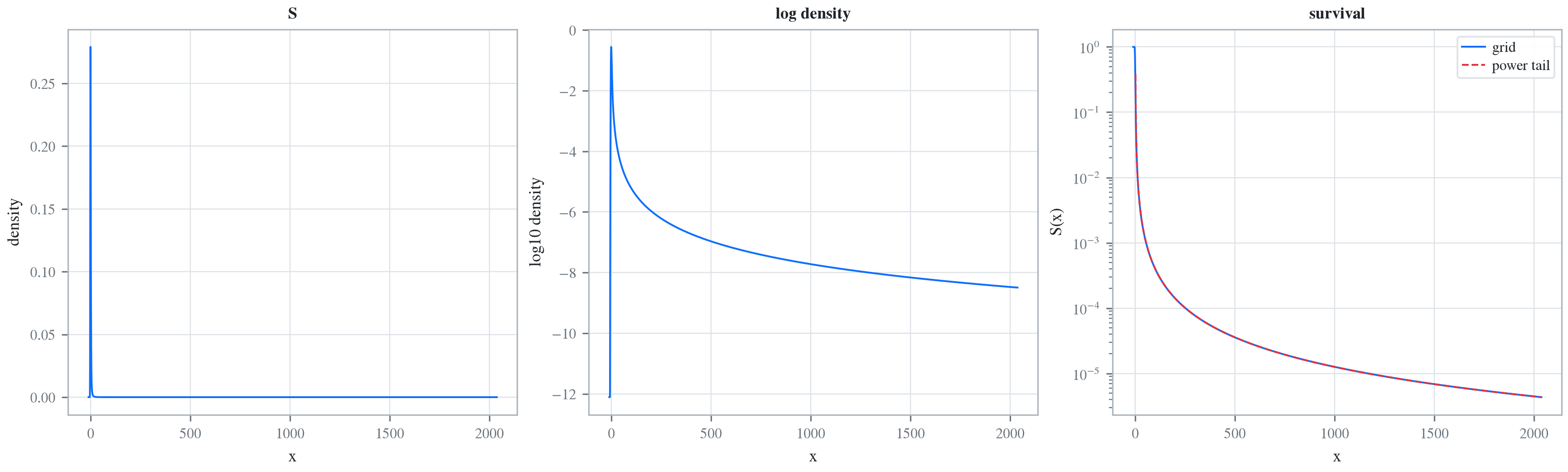
The method plot draws three panels: the density, its logarithm, and the survival function on a log axis with the power tail \(A x^{-\alpha}\) drawn in. The tail and the grid coincide out to the window’s end.

fig = s.plot()

Refused calls

A tilt below zero, or one that is not a number, is refused, as is a numeric tilt on a law with no power tail.

for bad in [-1, 'x']:
    try:
        s.update(tilt=bad)
    except ValueError as err:
        wprint(err)
try:
    AggregateCHF('G', 'gamma', shape=4, scale=25).update(tilt=8)
except ValueError as err:
    wprint(err)

tilt must be True, False or a number >= 0, got -1
tilt must be True, False or a number >= 0, got 'x'
G: tilt=8 on a gamma law, which has no power tail; such a law barely wraps, so
there is nothing for a tilt to damp. Use tilt=True or tilt=False.

Footnotes

1. From aggregate 1.28.0

2. From aggregate 1.30.0