Using stable

Stable laws with the stable statement and aggregate.stable.Stable

An \(\alpha\)-stable law is the only possible limit of a normalized sum of independent, identically distributed variables. When the summands have finite variance the limit is the normal, \(\alpha=2\). When they have a power tail \(\Pr(X>x)\sim cx^{-\alpha}\) with \(0<\alpha<2\), as a Pareto severity does, the limit is a stable law with index \(\alpha\). This result is the generalized central limit theorem.

A stable law has four parameters: the index \(\alpha\in(0,2]\), the skewness \(\beta\in[-1,1]\), the scale \(\gamma>0\) and the location \(\delta\). Two parameterizations are in common use, and they differ only in the location. In Nolan’s S1, the default here and in scipy, the characteristic function is \[ \log \mathsf{P}e^{itX} = -\gamma^\alpha|t|^\alpha\bigl(1 - i\beta\,\mathrm{sign}(t)\tan(\pi\alpha/2)\bigr) + i\delta_1 t \] for \(\alpha\ne1\), and the locations of a sum add. In S0 the location is \(\delta_0 = \delta_1 + \beta\gamma\tan(\pi\alpha/2)\), which is continuous in \(\alpha\). For \(1<\alpha<2\) the mean is \(\delta_1\).

The class aggregate.stable.Stable¹ represents a stable law. It can be created with the DecL statement stable. Without a name the statement stores nothing. With a name, as in stable x0 1.5 0, it stores the law in the recipe base under stable.x0, as described in Using stable names and arithmetic. It is used to approximate the aggregate loss of a large unit with a Pareto severity by its limit, which has a closed-form mean and tail constant. It is also used to combine the limits of several units with a common tail index. Using AggregateCHF with stable laws computes the same laws on a grid, accurately into the far tail.

stable 1.5 1 2 0                          # alpha beta scale loc, S1
stable 1.5 1 2 -2 s0                      # the same law in S0
stable 1000 claims sev 100 * lomax 1.5    # the stable limit of a Pareto book
stable x0 1.5 1 2 0                       # the first law, stored as stable.x0

import numpy as np
from aggregate import build, qd, __version__
from aggregate.stable import Stable
from style import wprint, refuse, figures, figure
figures()
print(__version__)

1.43.1

The stable statement

Printed, a Stable shows the law in both parameterizations, its mean, the probability that it exceeds the mean, and the constant \(A\) in its power tail \(\Pr(X>x)\sim Ax^{-\alpha}\). The object itself holds the S1 parameters.

x = build('stable 1.5 1 2 0')
wprint(x)
x

stable 1.5 1 2 0 = stable 1.5 1 2 -2 s0, mean 0, Pr(X>mean) 0.333333, Pr(X>x) ~
1.12838 x^-1.5

Stable(alpha=1.5, beta=1, scale=2, loc=0)

The S0 statement below describes the same law as the S1 statement above. The scale and location are optional, with defaults 1 and 0.

wprint(build('stable 1.5 1 2 -2 s0'))
wprint(build('stable 1.5 1'))

stable 1.5 1 2 0 = stable 1.5 1 2 -2 s0, mean 0, Pr(X>mean) 0.333333, Pr(X>x) ~
1.12838 x^-1.5
stable 1.5 1 1 0 = stable 1.5 1 1 -1 s0, mean 0, Pr(X>mean) 0.333333, Pr(X>x) ~
0.398942 x^-1.5

When \(\beta=1\) and \(1<\alpha<2\) the left tail is light and the mean is the \(1/\alpha\) quantile, so \(\Pr(X>\mathsf{P}X) = 1-1/\alpha\), here \(1/3\). A law with \(\beta<1\) has a power tail on both sides, and for \(\alpha\le1\) the mean does not exist.

wprint(build('stable 1.2 0'))
wprint(build('stable 0.5 1'))

stable 1.2 0 1 0 = stable 1.2 0 1 0 s0, mean 0, Pr(X>mean) 0.5, Pr(X>x) ~
0.277958 x^-1.2, Pr(X<-x) ~ 0.277958 x^-1.2
stable 0.5 1 1 0 = stable 0.5 1 1 1 s0, mean infinite, Pr(X>loc) 1, Pr(X>x) ~
0.797885 x^-0.5

Sums and scaling of stable laws

Independent stable laws with a common index \(\alpha\) add to a stable law with the same index: \(\gamma^\alpha\) adds, \(\beta\) is the \(\gamma^\alpha\)-weighted average, and in S1 the locations add. Scaling, negation and shifting stay in the family. For a real \(a\ne 0\), \(aX\) has skewness \(\mathrm{sign}(a)\beta\), scale \(|a|\gamma\) and location \(a\delta_1\), less \((2/\pi)\beta\gamma a\log|a|\) when \(\alpha=1\). The class Stable implements these rules with the operators +, -, * and /, and Using stable names and arithmetic shows the same operations in DecL. Each operand is an independent copy, so sum([x1, x1, x1]) is the sum of three independent copies of x1 and has a different scale from 3 * x1. The form 3 @ x1 returns the same sum.

x1 = Stable(1.5, 1, 2, 10)
x2 = Stable(1.5, -0.5, 1, -3)
wprint(x1 + x2)
wprint(3 * x1 - 5)
wprint(sum([x1, x1, x1]))
wprint(3 @ x1)

stable 1.5 0.608194 2.44726 7 = stable 1.5 0.608194 2.44726 5.51159 s0, mean 7,
Pr(X>mean) 0.384045, Pr(X>x) ~ 1.22811 x^-1.5, Pr(X<-x) ~ 0.299207 x^-1.5
stable 1.5 1 6 25 = stable 1.5 1 6 19 s0, mean 25, Pr(X>mean) 0.333333, Pr(X>x)
~ 5.86323 x^-1.5
stable 1.5 1 4.16017 30 = stable 1.5 1 4.16017 25.8398 s0, mean 30, Pr(X>mean)
0.333333, Pr(X>x) ~ 3.38514 x^-1.5
stable 1.5 1 4.16017 30 = stable 1.5 1 4.16017 25.8398 s0, mean 30, Pr(X>mean)
0.333333, Pr(X>x) ~ 3.38514 x^-1.5

The characteristic function of a sum of independent variables is the product of their characteristic functions. On a grid of \(t\) values the two sides differ only by rounding.

t = np.linspace(-2, 2, 9)
print(np.abs((x1 + x2).chf(t) - x1.chf(t) * x2.chf(t)).max())

1.1857187100668868e-16

The stable limit of a Pareto book

Take a Poisson count with mean \(\lambda\) and a severity with \(\Pr(X>x)=\theta^\alpha x^{-\alpha}(1+o(1))\), \(1<\alpha<2\). For large \(\lambda\) the aggregate is approximately \(S(\alpha, 1, \gamma, \lambda\mathsf{P}X; 1)\) with \(\gamma^\alpha = \lambda\theta^\alpha\Gamma(1-\alpha)\cos(\pi\alpha/2)\), which has exactly the aggregate’s mean and right tail constant \(\lambda\theta^\alpha\). The stable statement computes it from the count and severity.

s = build('stable 1000 claims sev 100 * lomax 1.5')
wprint(s)

stable 1.5 1 18452.7 200000 = stable 1.5 1 18452.7 181547 s0, mean 200000,
Pr(X>mean) 0.333333, Pr(X>x) ~ 1e+06 x^-1.5

The aggregate itself can be computed for comparison. The severity has infinite variance, so the grid is given explicitly. Validation fails the means because the grid truncates the tail: the computed aggregate mean is about 198,000 against 200,000.

a = build('agg Pareto 1000 claims sev 100 * lomax 1.5 poisson', bs=10, log2=18)
qd(a)

Aggregate object: Pareto. Frequency distribution poisson. Severity
lomax, [0, inf), power-law right tail. Updated with bucket size 10 and
log2 = 18. Validation: fails sev mean, agg mean.

           Mean     SD       CV     Skew        P01     Median        P99
X                                                                        
Freq       1000 31.623 0.031623 0.031623                                 
Sev      198.08 2176.8   10.989   411.09          0         60       2050
Agg  1.9808e+05  69002  0.34835   12.724 1.4284e+05 1.8618e+05 4.1113e+05

The quantiles of the aggregate and of its stable limit agree to within 4% at the 1% level and to within 1.5% from the 10% level up. The stable limit is lower at the bottom of the distribution, where the aggregate is still some way from its limit.

ps = [0.01, 0.1, 0.5, 2/3, 0.9, 0.99]
for p in ps:
    print(f'{p:6.3f} {a.q(p):12,.0f} {s.ppf(p):12,.0f}')

 0.010      142,840      137,793
 0.100      159,120      156,982
 0.500      186,180      186,775
 0.667      198,800      199,879
 0.900      237,970      239,595
 0.990      411,130      415,050

The densities are close across the body of the distribution. The stable limit puts a little more probability in the left tail, as the 1% quantiles show.

xs = np.linspace(s.ppf(0.001), s.ppf(0.995), 200)
fig, ax = figure('three-quarter')
df = a.density_df.loc[xs[0]:xs[-1]]
ax.plot(df.index, df.p_total / a.bs, label='aggregate')
ax.plot(xs, s.pdf(xs), ls='--', label='stable limit')
ax.set(xlabel='loss', ylabel='density', title='1000 claims of 100 * lomax 1.5')
ax.legend();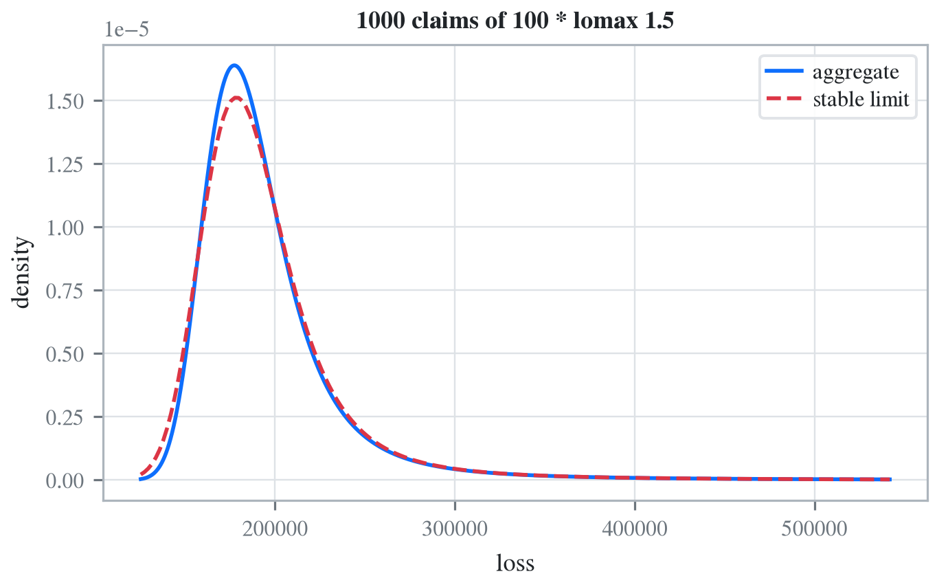

Distribution values and the far tail

The methods pdf, cdf, sf, ppf, isf and rvs of Stable call scipy.stats.levy_stable, which is accurate in the body of the distribution but not in the far tail. There the closed-form tail \(Az^{-\alpha}\) is the better guide. At \(z=5430\) the scipy survival function returns zero, and ppf(1 - 1e-6) returns 659, a point with survival probability \(2.4\times10^{-5}\), where the tail approximation gives about 5,420.

u = Stable(1.5, 1)
for z in [100, 659, 5430]:
    print(f'{z:6d} {u.sf(z):12.4e} {u.tail_constant * z ** -1.5:12.4e}')
print(u.ppf(1 - 1e-6), (u.tail_constant / 1e-6) ** (1 / 1.5))

   100   3.9894e-04   3.9894e-04
   659   2.3582e-05   2.3582e-05
  5430   0.0000e+00   9.9703e-07
659.2325672109375 5419.260701392888

Refused programs

An index outside \((0,2]\) is refused, as is a parameterization other than s0 or s1. The limit form needs a Pareto or Lomax severity with tail index strictly between 1 and 2, so a finite-variance Lomax and a lognormal are refused too.

refuse('stable 2.5 0',
       'stable 1.5 1 2 0 s2',
       'stable 1000 claims sev 100 * lomax 2.5',
       'stable 1000 claims sev lognorm 10 cv 1')

Stable: alpha must be in (0, 2], got 2.5
stable: the statement is 'stable alpha beta [scale [loc]] [s0|s1]'; the last
word must be s0 or s1, got 's2'
stable: the limit theorem form needs a plain pareto or lomax severity, `stable
<count> claims sev <scale> * lomax <alpha>`, but found the tail index 2.5, which
must be strictly between 1 and 2.
stable: the limit theorem form needs a plain pareto or lomax severity, `stable
<count> claims sev <scale> * lomax <alpha>`, but found severity 'lognorm'.

Footnotes

1. From aggregate 1.23.0