Using AggregateCHF

Distributions computed by inverting a characteristic function

The compound engine behind agg discretizes a severity, takes its FFT, applies the count’s probability generating function and inverts. Many infinitely divisible distributions¹ have an infinite claim count and no severity in the actuarial sense. They are easier to reach another way: they may have a closed-form characteristic function (chf) \(\varphi(t) = \mathsf{P}e^{itX}\). For these the first two steps are unnecessary. Sampling \(\varphi\) on the FFT’s frequency grid and inverting with one irfft gives the distribution directly. The object aggregate.characteristic_function.AggregateCHF² with corresponding DecL statement chfagg³ uses this alternative algorithm. It is a peer of Aggregate, not a subclass, and its frames, verdict, and members have Aggregate’s names and shapes, with the frequency and severity rows empty. It can be built for several families of distributions with closed form chfs. The examples here use three light-tailed families: norm, gamma, and invgauss. The positional numbers are the family’s shapes only, scipy’s where scipy has the law, and scale and location are arithmetic around it, c * FAMILY shapes + b, exactly as on an agg severity. A mean cv form takes the same arithmetic. The stable family, with heavy tails and tilting, has its own page, Using AggregateCHF with stable laws.

chfagg G 25 * gamma 4                      # scale and shape
chfagg G gamma 100 cv 0.5 hints{log2=14}   # the mean and cv form, with a grid hint
chfagg N as "Signed" 30 * norm + 100       # no shape; a signed window
chfagg I 400 * invgauss 0.25               # scipy's mu; also invgauss 100 cv 0.5

Two facts make the answers checkable. First, the engine returns bucket masses, not density samples: on the grid \(x_k = x_0 + kh\), with \(U\) uniform on \([-h/2, h/2]\), \(\Pr(X\in[x_k - h/2, x_k + h/2)) = h f_{X+U}(x_k)\) and \(\varphi_{X+U}(t) = \varphi_X(t)\,\mathrm{sinc}(th/2)\), so inverting \(\varphi\cdot\mathrm{sinc}\) gives the masses of the round discretization that agg uses, bucket for bucket. Second, the grid is sized from the law’s tails: with \(K(s) = \log\mathsf{P}e^{sX}\) the cumulant generating function, the Chernoff bound \(\Pr(X > x) \le \exp(K(s) - sx)\) gives an edge \(x_R = \inf_s (K(s) - \log\varepsilon)/s\) holding mass \(\varepsilon\) beyond it, and likewise on the left. Two errors remain, both reported: frequencies beyond \(\pi/h\) are dropped, costing about \(|\varphi(\pi/h)|\), and mass outside the window wraps onto it.

import numpy as np
import scipy.stats as ss
from aggregate import build, qd, __version__
from aggregate.characteristic_function import AggregateCHF
from style import wprint, GT, figures, figure, refuse
figures()
print(__version__)

1.43.1

A gamma law checked against scipy

The function build takes the DecL statement and returns the object updated. The constructor AggregateCHF takes the same law by name, with the full parameters from Python, and the method update sizes the grid and computes. The attribute info reports the grid chosen: for 25 * gamma 4 the window runs from 0 (the support bound) to about 1,000, with a bucket of 1/64, which is round_bucket of the window over \(2^{16}\) points.

g = build('chfagg G 25 * gamma 4')
qd(g)
wprint(g.info)

AggregateCHF object: G. Family 25 * gamma 4. Updated with bucket size
1/64 and log2 = 16. Validation: not unreasonable.

     Mean SD  CV Skew    P01 Median    P99
X                                         
Freq                                      
Sev                                       
Agg   100 50 0.5    1 20.578 91.797 251.12
aggregate object name    G
value_type               loss
claim count              n/a
frequency distribution   n/a
severity distribution    n/a
loss table               n/a
approximate              exact
bs                       1/64
log2                     16
padding                  n/a
sev_calc                 n/a
dsev_bucket              n/a
normalize                False
x_min                    0
x_max                    1,023.98
premium                  n/a
expected loss            100
loss ratio               n/a
P(X=0)                   2.11506e-16
validation_eps           0.0001
reinsurance              none
occurrence reinsurance   no reinsurance
aggregate reinsurance    no reinsurance
validation               not unreasonable
family                   gamma
parameters               25 * gamma 4
support                  0 to inf
scale                    50
total mass               1
outside mass             1.01e-12, below 0, above 1.01e-12
tilt                     (0, 0)
theta                    (0, 0)
edge error               n/a
truncation error         1.57e-15
transfer sigma           n/a
most negative bucket     -6.28e-17
buckets per scale        3.2e+03
checks                   5 ok
frequency tail           none: a characteristic function law
severity tail            none: a characteristic function law
aggregate tail           [0, inf), exponential right tail; not concentrated
                         (cv=0.5)
bounded                  False
id                       03F5E2DE

g2 = AggregateCHF('G', 'gamma', shape=4, scale=25)
g2.update()
print(np.abs(g.agg_density - g2.agg_density).max(), g.program, g2.program == '')

0.0 chfagg G 25 * gamma 4 True

The family includes a scipy reference, so the masses can be checked against the exact bucket probabilities \(F(x_k + h/2) - F(x_k - h/2)\). They agree to roundoff.

h, x = g.bs, g.xs
exact = g.family.reference.cdf(x + h / 2) - g.family.reference.cdf(x - h / 2)
print(f'{np.abs(g.agg_density - exact).max():.2e}')

6.66e-16

The same law through the compound engine is agg G dfreq [1] sev 25 * gamma 4, a fixed count of one claim. On a shared grid the two agree bucket for bucket, to about \(10^{-11}\).

a = build('agg G dfreq [1] sev 25 * gamma 4', log2=12, bs=1/4)
g.update(log2=12, bs=1/4)
print(f'{np.abs(a.density_df.p_total - g.density_df.p_total).max():.2e}')
qd(a)

1.29e-11
Aggregate object: G. Frequency distribution empirical. Severity gamma,
[0, inf), exponential right tail. Updated with bucket size 1/4 and log2
= 12. Validation: not unreasonable.

      Mean  SD  CV Skew  P01 Median    P99
X                                         
Freq     1   0   0                        
Sev    100  50 0.5    1 20.5  91.75 251.25
Agg    100  50 0.5    1 20.5  91.75 251.25

The normal and inverse Gaussian laws

The normal law is supported on the whole line, so its window is signed. The Chernoff edges for the mass budget sit 5 standard deviations either side of the mean; the bucket is rounded up to a power of two, and the width that rounding adds is split between the two sides, so the window runs from \(-156\) to \(356\), about 8.5 standard deviations each way. The printed percentiles are those of the law, from scipy.

n = AggregateCHF('N', 'norm', mean=100, sd=30)
n.update()
print(n.x_min, n.x_max, n.bs)
GT(n.summary_df)
print(ss.norm(100, 30).ppf([0.01, 0.5, 0.99]))

-156.0 355.9921875 0.0078125
[ 30.20956378 100.         169.79043622]

Every family with a mean and coefficient of variation has a mean cv form, written with form='cv'. The inverse Gaussian with mean 100 and cv 0.5 is the law with shape \(\lambda = \mu/\mathrm{cv}^2 = 400\); its scipy reference is invgauss(mu / lam, scale=lam).

i = AggregateCHF('I', 'invgauss', form='cv', mean=100, cv=0.5)
i.update()
wprint(i.family, i.family.reference.mean(), i.family.reference.var() ** 0.5 / 100)
GT(i.stats_df.loc['agg', ['mixed', 'empirical', 'error']])

FamilyInverseGaussian('invgauss 100 cv 0.5') 100.0 0.5

measure	mixed	empirical	error
ex1	100.0000	100.0000	-6.73e-09
ex2	12500.0000	12499.9993	-5.86e-08
ex3	1937500.0000	1937499.1939	-4.16e-07
mean	100.0000	100.0000	-6.73e-09
cv	0.5000	0.5000	-1.13e-07
skew	1.5000	1.5000	-2.85e-06

The Tweedie family at every admissible power

A Tweedie law with \(1 < p < 2\) is a compound Poisson with gamma severity, and the tweedie clause of an agg builds it that way (Using tweedie). The members with \(p > 2\) and \(p < 0\) are tilted stable laws with no severity and no count, which only the characteristic function reaches. The DecL statement chfagg T tweedie p mean dispersion⁴ covers every admissible \(p\) (not 1, a lattice law, and not between 0 and 1, where no law exists). For \(1 < p < 2\) the atom \(e^{-\lambda}\) at 0 is split out of \(\varphi\) before inversion and put back in the bucket at 0, so truncation does not ring around it; the skewness of every member is \(p\) times the coefficient of variation.

for p in [1.5, 2.5, -1]:
    t = build(f'chfagg T tweedie {p} 100 cv 0.5')
    m, var, skew = t.family.moments
    print(f'p={p:5}  mean {t.est_m:8.4f}  cv {t.est_cv:.5f}  skew {t.est_skew:.4f} = {p} * cv  atom {t.family.atom}')

p=  1.5  mean  99.9999  cv 0.50000  skew 0.7499 = 1.5 * cv  atom (0.0, 0.00033546262790251185)
p=  2.5  mean 100.0000  cv 0.50000  skew 1.2500 = 2.5 * cv  atom None
p=   -1  mean 100.0000  cv 0.50000  skew -0.5000 = -1 * cv  atom None

The normal inverse Gaussian, variance gamma, and tempered stable laws of finance are infinitely divisible, with a closed-form cumulant function and light tails on both sides. Each has its moments in closed form, and the grid reproduces them.

for prog in ['chfagg N 3 * norminvgauss 6 1.5 + 1', 'chfagg V variancegamma 0.2 0.5 -0.1', 'chfagg C temperedstable 1 5 10 0.5 + 2']:
    a = build(prog)
    m, var, skew = a.family.moments
    print(f'{a.family.name:15} mean {m:8.4f} {a.est_m:8.4f}  sd {var ** 0.5:.5f} {a.est_sd:.5f}  skew {skew:.4f} {a.est_skew:.4f}')

norminvgauss    mean   1.7746   1.7746  sd 1.28549 1.28549  skew 0.3112 0.3112
variancegamma   mean  -0.1000  -0.1000  sd 0.21213 0.21213  skew -0.6809 -0.6809
temperedstable  mean   1.7678   1.7678  sd 0.32755 0.32755  skew -0.5570 -0.5570

Validation and the truncation error

The table validation_df has the same shape as on an Aggregate, with the law’s moments against the grid’s, and the attribute validation_description uses the same words. The checks on the inversion itself, the mass outside the window, the truncation error \(|\varphi(\pi/h)|\), the most negative bucket, and the buckets per body scale, are lines of info, counted in its checks line and written out in validation_explanation. A clean law has the description not unreasonable. An exponential law, 25 * gamma 1, has a density jump at 0, so \(|\varphi(t)|\) decays only like \(1/t\): the truncation flag sets, and the ringing shows as a negative bucket and a mean a few parts in \(10^4\) off. A gamma shape of 3 or more decays fast enough.

e = build('chfagg E 25 * gamma 1')
wprint(e.validation_description)
GT(e.validation_df.loc[['Agg']])
print('\n'.join(ln for ln in e.info.splitlines() if ln.startswith(('truncation', 'most negative', 'checks'))))

fails agg mean, characteristic function truncated at pi / bs, lower bs
truncation error         9.95e-05
most negative bucket     -1.56e-05
checks                   3 ok, 2 flags: most negative bucket; truncation error

Choosing the grid of a chfagg

Rule A, the default, sizes the window from the tails and the bucket from log2. Rule C takes bs and log2 as given, with the left edge from the same rule, and 0 is always a grid point. The method grid_window shows the choice without computing. The method recommended_grid returns the smallest grid meeting coverage, truncation, and ten buckets per body scale. The table bs_window_df lays out the decision in the same columns as on an Aggregate, and the method sharpen audits it: a sound grid scoring under the target is confirmed and nothing runs, and otherwise the object moves toward the recommended grid, at most one log2 per call.

print(n.grid_window(log2=16))
print(n.grid_window(log2=12, bs=1/8))
print(n.recommended_grid())
GT(n.bs_window_df[['selected', 'x_min', 'x_max', 'bs', 'log2', 'coverage']])
wprint(n.sharpen().sharpen_description)

(0.0078125, 16, -156.0, (0.0, 0.0))
(0.125, 12, -156.0, (0.0, 0.0))
(8, 2.0)
Sharpen: not run, the grid already scores 0.00116 against a target of 0.5 and
its outside mass is within the budget.

Output tables and the plot of a chfagg

The table density_df has the same columns as on an Aggregate. The table tail_df is the return-period ladder, and tail_behavior_df gives the tail class on each side. The methods price, evaluate, and apply_distortion work as on an Aggregate. The method plot shows the density, its logarithm, and the survival function with the Chernoff bound drawn in.

GT(g.tail_df.tail(4))
GT(g.tail_behavior_df.loc[['aggregate'], ['min', 'max', 'left_tail', 'right_tail', 'cv']])

component	min	max	left_tail	right_tail	cv
aggregate	0	—	bounded	exponential	0.5000

fig = g.plot()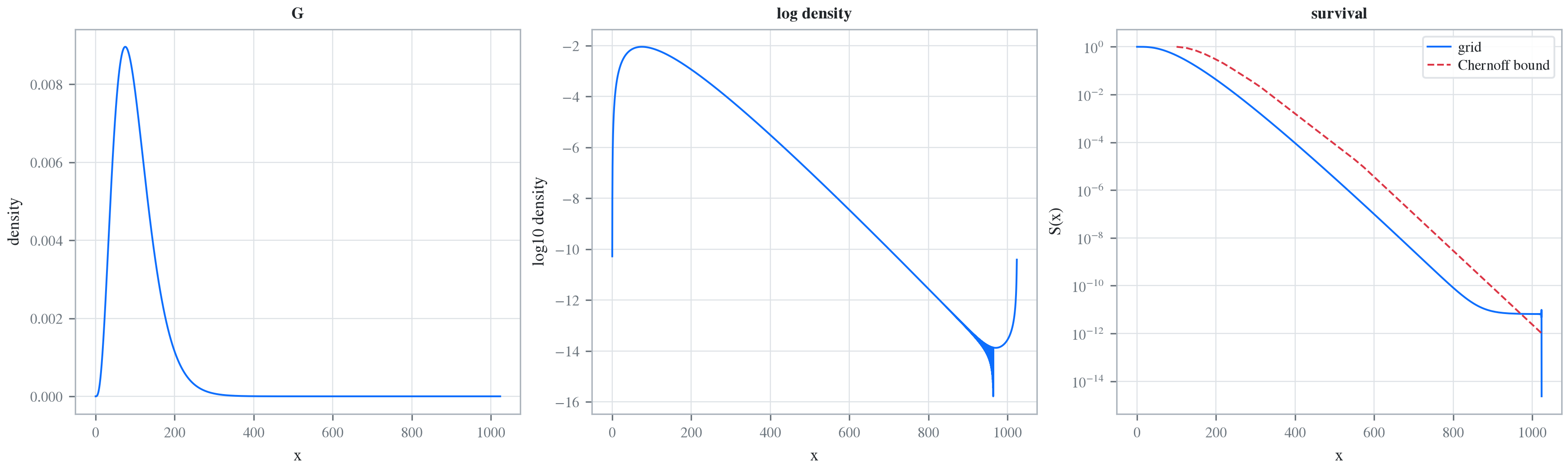

Refused calls

A number the family does not take is refused with the arithmetic form of the same law. An unknown family, a mean cv form on a family without one, a negative multiplier, and a numeric tilt on a law with no power tail are refused too.

refuse('chfagg G gamma 4 25', 'chfagg N norm 100 30', 'chfagg X lognorm 1 2',
       'chfagg X stable 1.5 cv 1', 'chfagg X -2 * gamma 4',
       lambda: g.update(tilt=8))

chfagg: gamma takes 1 shape, shape, got 2. Scale and location are arithmetic
around the law, as on an agg severity: write 'gamma 4 25' as '25 * gamma 4'.
chfagg: norm takes no shape (the standard law), got 2. Scale and location are
arithmetic around the law, as on an agg severity: write 'norm 100 30' as '30 *
norm + 100'.
chfagg: unknown family 'lognorm'; the families are stable, tweedie, norm, gamma,
invgauss, norminvgauss, variancegamma, temperedstable. The statement is 'chfagg
NAME [c *] LAW [+ b | - b], LAW one of stable alpha beta [s0|s1], tweedie p mean
dispersion, tweedie p mean cv c, norm, gamma shape, invgauss mu, norminvgauss a
b, variancegamma sigma nu theta, temperedstable C G M Y, or FAMILY mean cv c'.
DecL parse error at line 1, column 21: Unexpected 'cv'.
chfagg: the scale in 'c * gamma' must be positive, got -2; a reflection is not
supported (for a stable law, negate beta)
G: tilt=8 on a gamma law, which has no power tail; such a law barely wraps, so
there is nothing for a tilt to damp. Use tilt=True or tilt=False.

Footnotes

1. The gamma, lognormal, Pareto, stable, Poisson, and inverse Gaussian are infinitely divisible, amongst many others.

2. From aggregate 1.27.0

3. From 1.30.0

4. From aggregate 1.31.0