---
title: Using sliding scale commissions
subtitle: "Sliding scale ceding commissions on an aggregate quota share with the DecL slide clause"
categories: [reinsurance, variable feature, P&L]
date: last-modified
jupyter:
jupytext:
text_representation:
extension: .qmd
format_name: quarto
format_version: '1.0'
kernelspec:
display_name: Python 3 (ipykernel)
language: python
name: python3
---
A **sliding scale commission** is a ceding commission on a proportional treaty, usually a quota share, that falls as the loss ratio of the treaty rises. The reinsurer pays a high commission in a good year and a low one in a bad year, so the cedant keeps part of the variability of the business it cedes. The scale is a set of anchors, a commission rate $c_i$ at a ceded loss ratio $\lambda_i$, with the rate decreasing in the loss ratio. With ceded loss $A$ and a fixed ceded premium $P_C$, the ceded loss ratio is $\lambda = A/P_C$ and the commission is
$$
K = c(\lambda)\,P_C,
$$
where $c$ interpolates linearly between the anchors and is flat outside them, so the first and last anchors set the maximum and minimum commission.
In DecL the clause `slide <c> at <λ> and ...` decorates one layer of an `aggregate net of` program in place of the flat commission `cede`. The layer needs a `deposit`, `rol`, or `rate` premium to form the loss ratio. The sliding scale is one of the variable features of DecL, with [profit commissions](profit-commission.qmd), [loss corridors](loss-corridor.qmd), [swing rating](swing-rating.qmd), and [retro rating](retro-rating.qmd). A program takes at most one of them. The reinsurance features decorate aggregate covers only, and all take effect in a `pnl` or `xpnl` (see [Using pnl and xpnl](pnls.qmd)). The commission is booked in the expense column of the cover, `E` in `economic_ratios_df`, as a random credit to the cedant.
```decl
aggregate net of 50% po inf xs 0 rate 100% cede 0.25 as QS          # flat
aggregate net of 50% po inf xs 0 rate 100% slide 0.35 at 0.6 and 0.25 at 0.7 and 0.15 at 0.8 as QS
aggregate net of 50% po inf xs 0 rate 100% slide 30% at 55% and 20% at 75% as QS
```
The variable feature pages share one base book: premium 10,000 at a 70% loss ratio, a policy limit of 2,000, lognormal severity with mean 150 and CV 2.5, gamma mixed claim counts with mixing CV 0.25, and expenses of 25% of premium. The setup cell wraps the book in an `xpnl` with a slot for each reinsurance program.
```{python}
import numpy as np
import pandas as pd
from aggregate import build, qd, __version__
from style import wprint, GT, refuse, figures, figure
figures()
print(__version__)
book = '''agg Book
  10000 premium at 0.7 lr
  2000 xs 0
  sev lognorm 150 cv 2.5 {occurrence}
  mixed gamma 0.25 {aggregate}'''
program = '''xpnl {name}
  inherit premium
  less
    ''' + book + '''
  less
    0.25 premium expenses'''
def quota_share(name, terms):
    """The base book under a 50% quota share at a 100% rate with the given terms."""
    return build(program.format(name=name, occurrence='',
                 aggregate=f'aggregate net of 50% po inf xs 0 rate 100% {terms} as QS'))
```
## A sliding scale on a 50% quota share
The cover is a 50% quota share of the base book at 100% of the subject premium, so the ceded premium is 5,000 and the ceded loss ratio equals the gross loss ratio, with mean 70%. The scale pays 35% at a ceded loss ratio of 60%, 25% at the expected 70%, and 15% at 80%. The comparison is the same quota share with a flat 25% commission. The parsed terms of the cover are stored in the attribute `variable_terms` of the wrapped aggregate, `engine`.
```{python}
flat = quota_share('Flat', 'cede 0.25')
slide = quota_share('Slide', 'slide 0.35 at 0.6 and 0.25 at 0.7 and 0.15 at 0.8')
print(slide.engine.variable_terms)
qd(slide)
```
The `QS` step is the cover from the cedant's side: the ceded premium of 5,000 against the recovery and the commission, which together make the obligation row, with mean 4,792. Its `Net` row is the running net result, here the same as `All`. The ledger `economic_df` lists the commission as its own leg, with mean 1,292 and standard deviation 448. In the 1 in 100 bad year, column `κ01`, the commission is at its minimum, 750, and in the 1 in 100 good year, `κ99`, at its maximum, 1,750.
```{python}
GT(slide.economic_df.loc['QS', ['EX', 'SD', 'κ01', 'κ50', 'κ99']], float_format=',.0f')
```
The mean commission, 1,292, is 25.85% of the ceded premium, more than the 25% paid at the expected loss ratio. Between the end anchors the rate falls one point per point of loss ratio, so $c(\lambda) = 0.95 - \lambda + (\lambda - 0.8)^+ - (0.6 - \lambda)^+$ and, since $\mathsf{P}\lambda = 0.7$, the mean rate is $\mathsf{P}c(\lambda) = 0.25 + \mathsf{P}(\lambda - 0.8)^+ - \mathsf{P}(0.6 - \lambda)^+$. The loss ratio is skewed to the right, so the floor at 15% cuts off a longer tail than the cap at 35%, and the last two terms add 0.85 points.
## Commission and net result against the flat commission
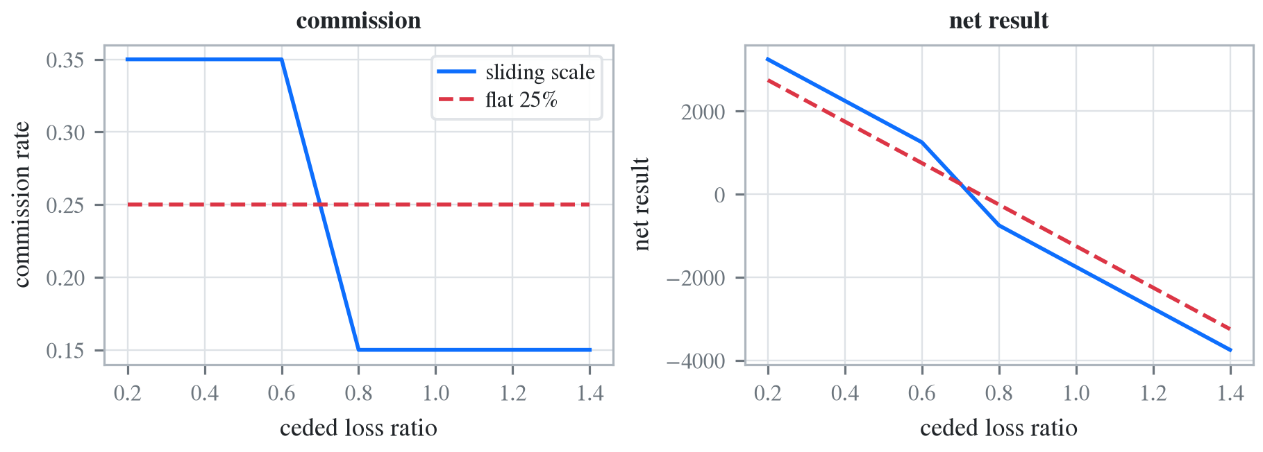
The commission rate and the cedant's net result are both functions of the ceded loss ratio. The gross loss is $10{,}000\lambda$ and the recovery $5{,}000\lambda$, so the net result, premium less expense and ceded premium, plus commission and recovery, less gross loss, is $2{,}500 + 5{,}000(c(\lambda) + \lambda) - 10{,}000\lambda$. The left panel shows the two commission rates and the right panel the two net results.
```{python}
lr = np.linspace(0.2, 1.4, 241)
rates = {'sliding scale': slide.engine.variable_terms.phi(lr), 'flat 25%': np.full_like(lr, 0.25)}
fig, (ax0, ax1) = figure('full', cols=2)
for (k, c), ls in zip(rates.items(), ['-', '--']):
    ax0.plot(lr, c, ls=ls, label=k)
    ax1.plot(lr, 10000 - 2500 - 5000 + 5000 * (c + lr) - 10000 * lr, ls=ls, label=k)
ax0.set(xlabel='ceded loss ratio', ylabel='commission rate', title='commission')
ax1.set(xlabel='ceded loss ratio', ylabel='net result', title='net result')
ax0.legend();
```
Between 60% and 80% the scale takes back one point of commission per point of loss ratio, so the net result falls at twice the slope of the flat cover: the cedant bears the whole movement of the ceded loss ratio in the band, on top of its retained half. Outside the band the two lines are parallel, the sliding scale 500 above the flat cover in good years and 500 below it in bad ones. The table compares the two covers over the whole distribution, with `P01` the 1 in 100 bad result.
```{python}
df = pd.DataFrame({k: [-x.economic_ratios_df.loc['QS', 'E'], x.est_m, x.est_sd, x.q(0.01), x.cdf(0)]
                   for k, x in {'flat 25%': flat, 'sliding scale': slide}.items()},
                  index=['commission', 'mean', 'SD', 'P01', 'Pr(loss)']).T
df.index.name = 'cover'
GT(df, float_format=',.0f', ratio_cols=['Pr(loss)'])
```
The sliding scale adds 42 to the mean result, from the 0.85 points of extra expected commission, and costs 500 in the 1 in 100 year, where `P01` falls from $-3{,}536$ to $-4{,}036$. The standard deviation (SD) of the net result rises from 1,352, half the gross 2,704, to 1,754, and the probability of a loss, a result of zero or less, from 38.5% to 41.9%.
## Refused programs
A sliding scale replaces the flat commission across its aggregate program, so a `cede` on the same layer or on another aggregate layer is refused. A scale whose commission rises with the loss ratio is not a sliding scale and is refused too.
```{python}
refuse(lambda: quota_share('R1', 'cede 0.25 slide 0.35 at 0.6 and 0.15 at 0.8'),
       lambda: quota_share('R2', 'slide 0.35 at 0.6 and 0.15 at 0.8 and 2000 xs 8000 rate 6% cede 0.2'),
       lambda: quota_share('R3', 'slide 0.15 at 0.6 and 0.35 at 0.8'))
```