Using bivariate

Joint distribution of two aggregates sharing one claim count, coupled by a copula or a discrete bivariate severity

A bivariate aggregate is the joint distribution of two aggregate losses that share one claim count. Each of the \(N\) claims produces a pair \((A_i, B_i)\), and the two totals are \(X = A_1 + \dots + A_N\) and \(Y = B_1 + \dots + B_N\). Loss and allocated expense (ALAE) on the same claims are the standard example, and damage to two lines from the same storms is another. The DecL kind bivariate, with the alias bv, builds the joint law of \((X, Y)\) as a BivariateAggregate, from which the marginals, the law of the sum \(X + Y\), and any conditional law follow.

The per-claim pair has a joint probability matrix \(S\) on a two-dimensional grid. With \(G_N(z) = \mathsf{P}z^N\) the probability generating function of \(N\), applied entry by entry, the joint aggregate density is \(\mathrm{FFT2}^{-1}(G_N(\mathrm{FFT2}(S)))\), the ordinary FFT method with two-dimensional transforms. The dependence between \(X\) and \(Y\) has two sources, \[ \mathrm{cov}(X, Y) = \mathsf{P}N\,\mathrm{cov}(A, B) + \mathrm{var}(N)\,\mathsf{P}A\,\mathsf{P}B, \] the dependence within a claim and the shared count. For a Poisson count with mean \(\lambda\) the covariance is \(\lambda\,\mathsf{P}AB\).

The per-claim matrix \(S\) is given in one of two ways. Two component agg statements, each with the one-claim frequency dfreq [1] (or dfreq [0 1] [0.7 0.3] for a component that only 30% of claims reach), set the marginal severities, and a copula clause couples them: gumbel or clayton with Kendall’s tau, normal with the correlation, or fgm with Spearman’s rho. With no copula clause, or copula independent, the pair is independent within a claim. Alternatively, dbvsev gives \(S\) directly, the two-dimensional analog of dsev: dense, as two outcome vectors and a matrix whose rows are indexed by the \(x\) outcome, or sparse, as a list of [x y p] triples. The shared count is a claim count with a frequency, Poisson by default, or a dfreq. The same machinery underlies the reinsurance views in Using grossnet, grossceded and netceded and the shared-event model in Using clash.

bivariate NAME 10 claims agg A dfreq [1] sev ... agg B dfreq [1] sev ... copula gumbel 0.4 poisson
bv NAME dfreq [1 2] [0.5 0.5] agg A dfreq [1] sev ... agg B dfreq [1] sev ...   # independent
bv NAME 3 claims dbvsev [1 2] [1 2] [[0.4 0.1] [0.1 0.4]] poisson               # dense
bv NAME dfreq [2] dbvsev [[1 1 0.4] [1 2 0.1] [2 1 0.1] [2 2 0.4]]              # sparse
bv NAME dfreq [2] dbvsev [1 2] [1 2]                                             # uniform

import pandas as pd
from aggregate import build, qd, __version__
from style import wprint, GT, refuse, figures, figure
figures()
print(__version__)

1.60.1

Loss and ALAE coupled by a copula

The example has ten claims a year, Poisson, each with a lognormal loss of mean 100 and coefficient of variation (CV) 1 and a gamma ALAE of mean 25 and CV 0.8. A Gumbel copula with Kendall’s tau 0.4 makes a large loss likely to come with a large expense. The program is written with a placeholder for the copula, so that it can be varied below. The function qd shows the grid and the realized correlation of \(X\) and \(Y\), then one row for each marginal and a total row for \(X + Y\).

program = '''bivariate LossALAE 10 claims
  agg Loss dfreq [1] sev lognorm 100 cv 1
  agg ALAE dfreq [1] sev gamma 25 cv 0.8
  copula {} poisson'''
b = build(program.format('gumbel 0.4'))
qd(b)

BivariateAggregate(name='LossALAE', units=['Loss', 'ALAE'],
Copula('gumbel', tau=0.4 -> tau=0.4000), shape=(4096, 256), corr=0.8384)

        Mean     SD      CV    Skew  P01  Median  P99
unit                                                 
Loss    1000 447.23 0.44723 0.89435  228     940 2316
ALAE  249.91 101.35 0.40553 0.56276   60     240  525
total 1249.9 535.06 0.42808 0.80253  300    1185 2795

The table dependency_df gives the covariance and correlation per claim (Sev) and in aggregate (Agg), with the Kendall tau of the copula. The correlation rises from 0.648 per claim to 0.838 in aggregate, because the shared count adds \(\lambda\,\mathsf{P}A\,\mathsf{P}B = 10 \times 100 \times 25 = 25{,}000\) to the covariance.

GT(b.dependency_df, float_format=',.3f')

level	cov	corr	tau
Sev	1,301.016	0.648	0.400
Agg	38,001.287	0.838	—

Effect of the dependence on the sum

The same pair is built below under three copulas with the same marginals, and the table shows the correlations and the law of the total. Under independent the loss and ALAE of a claim are independent, yet the aggregate correlation is 0.551, close to the \(25{,}000/(447.2 \times 101.2) = 0.552\) of the formula; the small gap is discretization. The Clayton copula concentrates dependence among small claims and the Gumbel among large ones, so with the same tau the Gumbel raises the 1 in 100 total, P99, and its tail value at risk, TVaR99, the most.

rows = {}
for cop in ['independent', 'clayton 0.4', 'gumbel 0.4']:
    bc = build(program.format(cop))
    d, t = bc.dependency_df, bc.total
    rows[cop] = [round(d.loc['Sev', 'corr'], 6) + 0, d.loc['Agg', 'corr'],
                 t.mean(), bc.summary_df.loc['total', 'SD'], t.q(0.99), t.tvar(0.99)]
df = pd.DataFrame.from_dict(rows, orient='index', columns=[
    'corr per claim', 'corr aggregate', 'mean', 'SD', 'P99', 'TVaR99'])
df.index.name = 'copula'
GT(df, float_format=',.1f', formatters={'corr per claim': '{x:.3f}',
                                        'corr aggregate': '{x:.3f}'})

copula	corr per claim	corr aggregate	mean	SD	P99	TVaR99
independent	0.000	0.551	1,249.9	510.2	2,700	3,023.6
clayton 0.4	0.326	0.696	1,249.9	522.8	2,735	3,063.6
gumbel 0.4	0.648	0.838	1,249.9	535.1	2,795	3,141.2

The column independent of stats_df gives the moments that \(X + Y\) would have if \(X\) and \(Y\) were independent, as they are with separate claim counts. Its standard deviation is 458.5, against 510.2 with the shared count and independent pairs, and 535.1 with the Gumbel copula as well.

s = b.stats_df.loc['agg']
print(s.loc['cv', 'independent'] * s.loc['mean', 'independent'])

458.53026072441526

The marginals and the total of a bivariate aggregate

The method marginal(axis) returns the law of one axis, selected by number or by name. The attribute total returns the law of \(X + Y\). Each is a distribution on its grid with mean, q, tvar, and cdf. Each marginal reproduces the standalone aggregate of its component. Below, the loss marginal is compared with the ordinary agg with the same count and severity: the means agree, and the 99th percentiles, 2,316 and 2,314.5, agree to within the bucket size of the loss axis of the joint grid, 4.

m = b.marginal('Loss')
loss = build('agg Loss 10 claims sev lognorm 100 cv 1 poisson')
print(b.bs)
print(m.mean(), loss.est_m)
print(m.q(0.99), loss.q(0.99))

[4.0, 5.0]
999.9998535035895 999.9999941986528
2316.0 2314.5

The method plot draws the joint per-claim severity \(S\) on the left and the joint aggregate density on the right, as filled contours. The grid extends far into the tail, so the axis limits are set after the call to show the bulk of each law.

fig, (ax0, ax1) = figure('full', cols=2)
b.plot(axs=(ax0, ax1))
ax0.set(xlim=[0, 400], ylim=[0, 100])
ax1.set(xlim=[0, 3000], ylim=[0, 600]);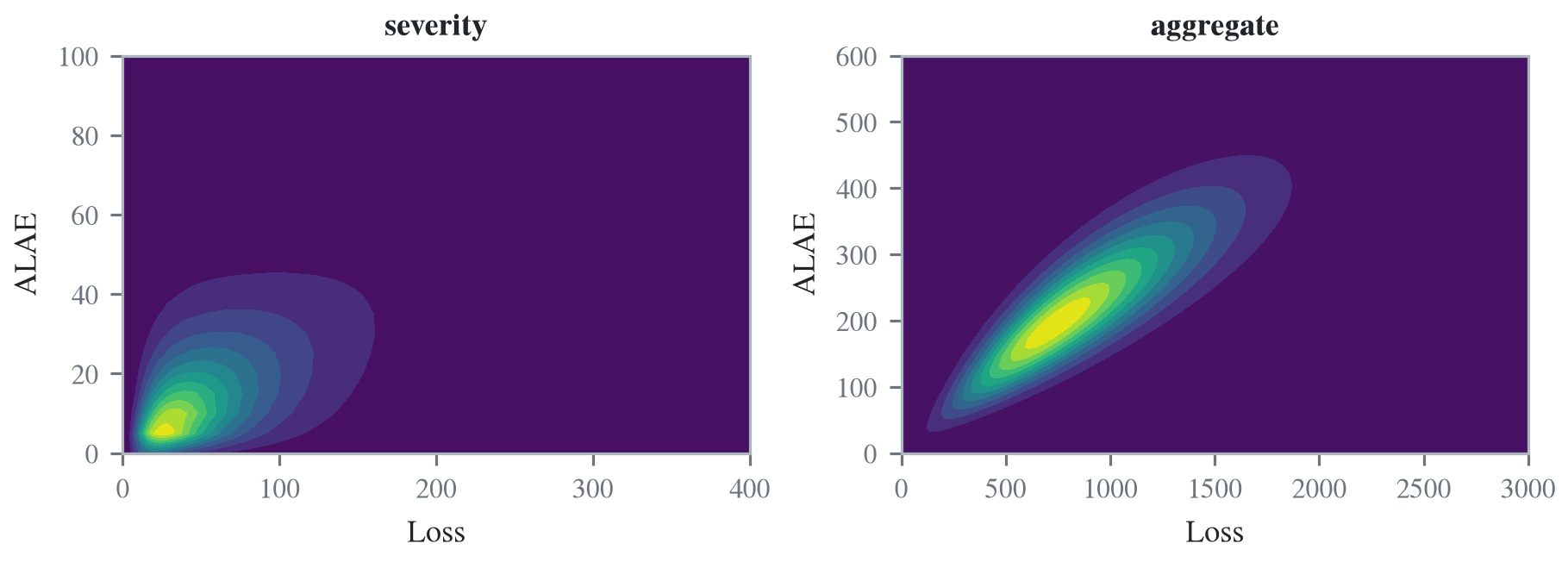

A discrete bivariate severity

With dbvsev the joint per-claim law is given outright. Below, there are exactly two claims, each a pair on \(\{1, 2\}^2\) whose components are equal with probability 0.8, given once as a dense matrix and once as sparse triples. The two forms give the same joint law, and density_df shows it with the \(x\) outcomes as the rows. By hand, \(X = Y = 3\) needs a 1 and a 2 on each axis: the pairs \((1, 1)\) and \((2, 2)\) in either order, \(2 \times 0.4^2 = 0.32\), or \((1, 2)\) and \((2, 1)\), \(2 \times 0.1^2 = 0.02\), for a total of 0.34.

dense = build('bv Dense dfreq [2] dbvsev [1 2] [1 2] [[0.4 0.1] [0.1 0.4]]')
sparse = build('bv Sparse dfreq [2] dbvsev [[1 1 0.4] [1 2 0.1] [2 1 0.1] [2 2 0.4]]')
print(abs(dense.density - sparse.density).max())
GT(dense.density_df.loc[2:4, 2:4], float_format='.4f')

0.0

X	2.0	3.0	4.0
2	0.1600	0.0800	0.0100
3	0.0800	0.3400	0.0800
4	0.0100	0.0800	0.1600

The per-claim correlation is \(0.15/0.25 = 0.6\), and with a fixed count the aggregate correlation is the same. A Poisson count with mean 3 adds the shared count term and raises it to \(\mathsf{P}AB/\mathsf{P}A^2 = 2.4/2.5 = 0.96\).

pois = build('bv Pois 3 claims dbvsev [1 2] [1 2] [[0.4 0.1] [0.1 0.4]] poisson')
print(dense.corr, pois.corr)

0.5999999999999979 0.9599999992543694

Refused programs

A bivariate has exactly two components, a copula parameter must lie in the range of its kind, the copula kind must be one of those listed in the message, and a dbvsev matrix may not have negative entries. A pinned grid must hold every dbvsev outcome, and the message gives the log2 that does.

import warnings
two = 'agg A dfreq [1] sev gamma 10 cv 1 agg B dfreq [1] sev gamma 10 cv 1'
with warnings.catch_warnings():
    warnings.simplefilter('ignore')    # R5 warns that the pinned grid is short, then refuses
    refuse(f'bv R1 10 claims {two} agg C dfreq [1] sev gamma 10 cv 1 poisson',
           f'bv R2 10 claims {two} copula gumbel 1.4 poisson',
           f'bv R3 10 claims {two} copula student 0.4 poisson',
           'bv R4 dfreq [2] dbvsev [1 2] [1 2] [[0.6 -0.1] [0.1 0.4]]',
           lambda: build('bv R5 dfreq [2] dbvsev [10 20 30] [10 20]', bs=1, log2=(4, 4)))

bivariate (copula) requires exactly two components; got 3
gumbel copula: tau must be in [0, 1), got 1.4
Unknown copula kind 'student'; available: ['clayton', 'fgm', 'gumbel',
'independent', 'normal', 'shuffle']
dbvsev: probability matrix has negative entries.
axis 0 needs log2 >= 5 at bs 1 to hold the atom 30; log2 4 was given