Using eventual_ruin

Eventual ruin at a stated margin and capital with Aggregate.eventual_ruin

An insurer with initial surplus \(u\), premium rate \(c\), and claims \(X_i\) has surplus \(U(t) = u + ct - \sum_{i\le N(t)}X_i\) at time \(t\), and is ruined at the time \(\tau = \inf\{t : U(t)<0\}\). The probability of eventual ruin is \(\psi(u) = \Pr(\tau<\infty)\). The premium rate is \(c = (1+\rho)\mathsf{P}X/\mathsf{P}W\), where \(W\) is the wait between claims and the margin \(\rho\) is the ratio of premium margin to expected loss. The methods pollaczeck_khinchine and wiener_hopf, described in Using pollaczeck_khinchine and wiener_hopf, compute the whole function \(\psi\). The method Aggregate.eventual_ruin evaluates it at a single surplus, and is used to find the ruin probability at a given capital or the capital at a given ruin probability.

The method Aggregate.eventual_ruin¹ takes the margin either as \(\rho\) or as the loss ratio \(1/(1+\rho)\), and the capital either as a target ruin probability \(p\) or as a surplus \(u\). It computes the exact \(\psi(u)\), by pollaczeck_khinchine for a Poisson count and wiener_hopf for a renewal count, checks it by simulating surplus paths of the same discretized model, and returns a RuinResult. The simulation also records \(\tau\) on each ruined path. These simulated times are the library’s only information on the time to ruin; there is no finite-horizon ruin probability \(\psi(u, t)\).

For exponential claims with mean \(m\) and Poisson arrivals at rate \(\lambda\), the Lundberg exponent, or adjustment coefficient, is \(R = \rho/((1+\rho)m)\), \(\psi(u) = e^{-Ru}/(1+\rho)\), and the mean time to ruin given ruin is \[ \mathsf{P}(\tau \mid \tau<\infty) = \frac{u + (1+\rho)m}{\rho c}, \qquad c = (1+\rho)\lambda m. \] Under the Lundberg conjugate measure ruin is certain and the claims exceed the premium at rate \(\rho c\), so by Wald’s identity the mean ruin time under that measure is \(u\) plus the mean deficit at ruin, divided by \(\rho c\). The deficit is exponential with mean \((1+\rho)m\) and independent of \(\tau\), so the law of \(\tau\) given ruin is the same under both measures. The examples use exponential claims with mean 1, and either a Poisson count of 10 claims a year, where these closed forms apply, or gamma waits with mean 2.

agg Po 10 claims sev expon poisson          # pollaczeck_khinchine, Lundberg rows
agg Ga 10 years sev expon wait gamma 2      # wiener_hopf

import numpy as np
from aggregate import build, qd, __version__
from aggregate.pedagogy import ruin_example
from aggregate.exhibits import exhibit_frames
from aggregate.charts import build_chart_doc
from style import wprint, GT, refuse, figures
figures()
print(__version__)

1.51.0

Ruin probability at a stated margin and capital

For the Poisson aggregate at a margin of 20%, the call eventual_ruin(rho=0.2, p=0.05) finds the surplus with a 5% ruin probability, 16.87. The attribute ruin_df of the result is a one-column table of the margin, as \(\rho\), as a loss ratio, and as a premium rate, the means of \(X\) and \(W\), the resolved surplus, the exact and simulated \(\psi\) with the details of the simulation, and, for a Poisson count, the Lundberg exponent and the bound \(e^{-Ru}\). With 1000 paths the simulated \(\psi\), 0.062, is within two standard errors of the exact 0.050.

po = build('agg Po 10 claims sev expon poisson')
r = po.eventual_ruin(rho=0.2, p=0.05)
print(r.ruin_df)

                             value
frequency kind             poisson
safety loading rho             0.2
loss ratio                0.833333
premium rate c           11.999998
mean severity E[X]             1.0
mean wait E[W]                 0.1
initial surplus u        16.865234
psi(u) exact              0.049996
psi(u) simulated             0.062
sim std error             0.007626
sim trials                    1000
sim ruins                       62
sim horizon (claims)          1254
seed                      20260905
Lundberg exponent R       0.166667
Lundberg bound exp(-Ru)   0.060153

At the resolved surplus the closed form is within \(2\times10^{-4}\) of the computed \(\psi\), which includes the discretization error of pollaczeck_khinchine. For exponential claims the Lundberg bound is exactly \((1+\rho)\psi(u)\).

R = 0.2 / 1.2
print(f'psi    closed form {np.exp(-R * r.u) / 1.2:.6f}   computed {r.psi:.6f}')
print(f'bound  closed form {np.exp(-R * r.u):.6f}   ruin_df  {r.ruin_df.value.iloc[-1]:.6f}')

psi    closed form 0.050127   computed 0.049996
bound  closed form 0.060152   ruin_df  0.060153

The simulation uses 1000 paths and a fixed seed by default, so a repeated call gives the same result. The argument seed=None draws a fresh seed and records it. The fields rho, u, psi, psi_sim, se_sim, and seed of the result contain the main values in ruin_df. The call below states the margin as a loss ratio of 0.8, so \(\rho = 0.25\), and the capital as a surplus of 10, with ten times as many paths. The simulated \(\psi\), 0.1115, is about one standard error from the exact 0.1081.

r2 = po.eventual_ruin(lr=0.8, u=10, n_sims=10_000)
print(f'rho {r2.rho:.4f}  u {r2.u}  psi {r2.psi:.6f}  '
      f'simulated {r2.psi_sim:.4f} ({r2.se_sim:.4f})  seed {r2.seed}')

rho 0.2500  u 10  psi 0.108057  simulated 0.1115 (0.0031)  seed 20260905

Ruin probability for a renewal count

For a renewal count, here gamma waits with mean 2, the method eventual_ruin uses wiener_hopf. Its ruin_df has no Lundberg rows. At a margin of 20% the surplus for a 1% ruin probability is 20.02, and 9 of the 1000 simulated paths are ruined.

ga = build('agg Ga 10 years sev expon wait gamma 2')
r3 = ga.eventual_ruin(rho=0.2, p=0.01)
print(r3.ruin_df)

                          value
frequency kind          renewal
safety loading rho          0.2
loss ratio             0.833333
premium rate c              0.6
mean severity E[X]          1.0
mean wait E[W]              2.0
initial surplus u     20.019531
psi(u) exact           0.009997
psi(u) simulated          0.009
sim std error          0.002986
sim trials                 1000
sim ruins                     9
sim horizon (claims)        973
seed                   20260905

Sample paths and the time to ruin

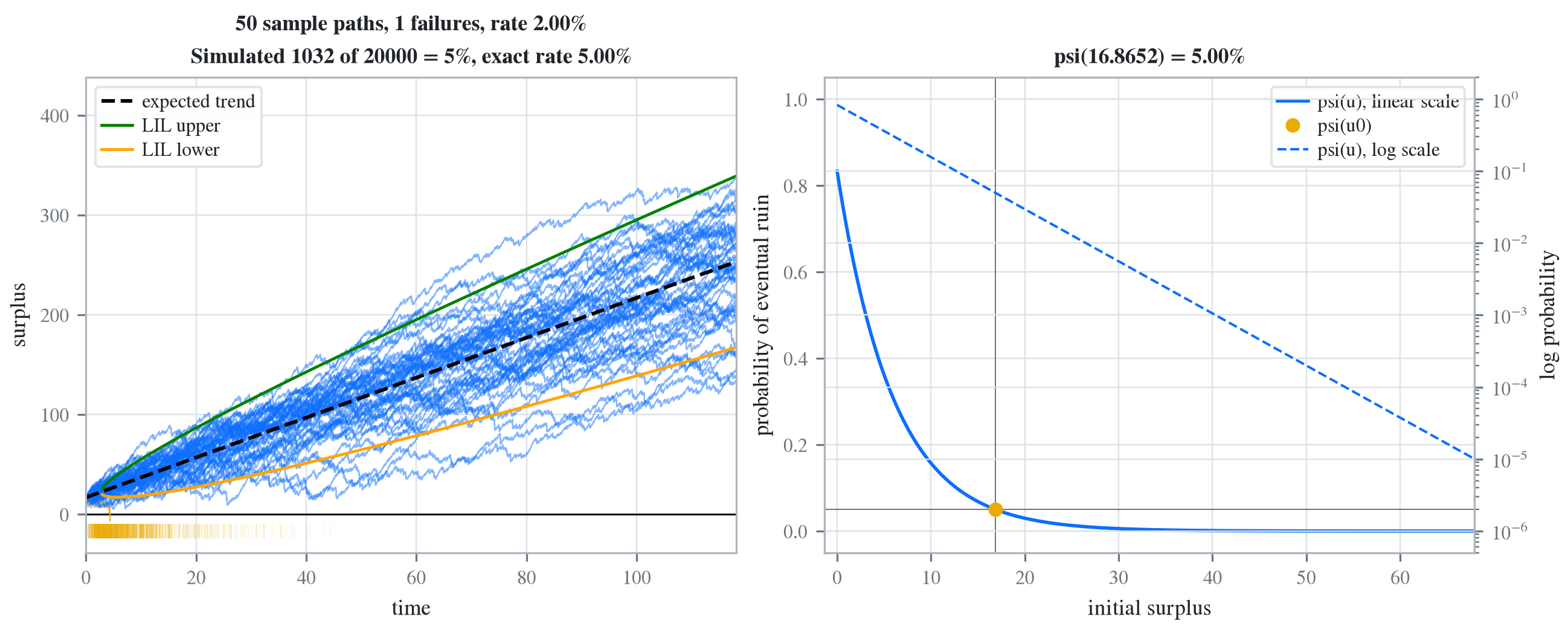
The ruin exhibit and the ruin chart present an eventual_ruin calculation in the aggregate Loss Lab, the browser application. The exhibit contains ruin_df, and the chart shows fifty sample paths and the \(\psi\) curve. The function pedagogy.ruin_example draws the same figure with matplotlib, from the same simulation, and returns a summary that includes the mean time to ruin given ruin.

name, frame, meta = exhibit_frames(r, 'ruin')[0]
print(name, frame.equals(r.ruin_df))
wprint(meta['caption'])
doc = build_chart_doc(po, 'ruin', rho=0.2, p=0.05)
wprint(*[p.title for p in doc.panels], sep='\n')

ruin_df True
One eventual-ruin reading: the premium margin stated as safety loading, loss
ratio and premium rate, the model moments, the resolved initial surplus, and the
exact probability of eventual ruin there beside a simulated check with its
standard error. Poisson books add the Lundberg exponent and bound when the
adjustment equation has a root on the grid.
50 sample paths, 3 ruined; simulated 62 of 1000 = 6.2%, exact 5.0%
psi(16.8652) = 5.00%

The left panel of the figure shows sample paths with the expected trend, a band from the law of the iterated logarithm, and a rug of simulated ruin times. The right panel shows \(\psi(u)\). Of 20,000 simulated paths 1,032 are ruined, and their mean time to ruin, 7.74, is about one standard error (some 0.21) above the closed form, 7.53.

summary, fig = ruin_example(po, 0.2, r.u, n_sims=20_000, seed=1)
fig.set_size_inches(9, 3.6)
rows = ['psi(u0) exact', 'psi(u0) simulated', 'sim std error', 'mean ruin time | ruin']
print(summary.loc[rows])
print(f'closed form mean time to ruin {(r.u + 1.2) / (0.2 * 12):.4f}')

                          value
psi(u0) exact          0.049996
psi(u0) simulated        0.0516
sim std error          0.001564
mean ruin time | ruin  7.739487
closed form mean time to ruin 7.5272

Refused calls

The method eventual_ruin requires exactly one positive margin, as rho or as a loss ratio lr below 1, and exactly one capital, as p or as a surplus u within the grid. The count must be Poisson or renewal.

nb = build('agg Nb 10 claims sev expon negbin 0.5')
refuse(lambda: po.eventual_ruin(rho=0, p=0.05),
       lambda: po.eventual_ruin(rho=0.2, lr=0.8, p=0.05),
       lambda: po.eventual_ruin(rho=0.2),
       lambda: po.eventual_ruin(lr=1.2, p=0.05),
       lambda: po.eventual_ruin(rho=0.2, u=1000),
       lambda: nb.eventual_ruin(rho=0.2, p=0.05))

net profit condition requires rho > 0, got 0
exactly one of rho and lr is required
exactly one of p and u is required
loss ratio must be in (0, 1), got 1.2
u0 = 1000 lies beyond the represented grid top 127.998
no eventual-ruin solver for a 'negbin' frequency: need poisson
(pollaczeck_khinchine) or renewal (wiener_hopf)

Footnotes

1. From aggregate 1.0