Using renewal counts

Renewal claim counts with a years exposure and the wait and dwait clauses

A Poisson claim count is the count of a process whose waiting times between claims are exponential. A renewal count keeps the independence and drops the exponential: the waits \(W_1, W_2,\dots\) are independent and identically distributed with mean \(\mu\), variance \(\sigma^2\), and third central moment \(\mu_3\). With \(S_k = W_1+\dots+W_k\) the count over \([0,T]\) is \(N(T) = \max\{k : S_k\le T\}\), so \(\{N(T)\ge k\} = \{S_k\le T\}\) and \(\Pr(N(T)=k) = F^{*k}(T) - F^{*(k+1)}(T)\), where \(F\) is the wait distribution. The renewal count is the claim count of the Sparre-Andersen risk model, and the method Aggregate.wiener_hopf computes its probability of eventual ruin, as described in Using pollaczeck_khinchine and wiener_hopf.

For a nonlattice wait law with a finite third moment, renewal theory gives \[ \mathsf{P}N(T) = \frac{T}{\mu} + \frac{\sigma^2-\mu^2}{2\mu^2} + o(1), \qquad \mathrm{Var}\,N(T) = \frac{\sigma^2 T}{\mu^3} + \frac{1}{12} + \frac{5\sigma^4}{4\mu^4} - \frac{2\mu_3}{3\mu^3} + o(1), \] so the index of dispersion \(\mathrm{Var}\,N/\mathsf{P}N\) tends to \(\sigma^2/\mu^2\), the squared coefficient of variation (CV) of the wait. Regular waits, with CV below 1, give an underdispersed count, and bursty waits, with CV above 1, an overdispersed one. The library computes the count probabilities from the convolution powers \(F^{*k}\) by FFT, not from these expansions.

A T years exposure¹ paired with a wait or dwait clause in place of the frequency gives a renewal count. The clause wait accepts any severity specification, applied on the time axis, including a layer such as wait 2 xs 1 expon. The clause dwait takes outcomes and probabilities like dsev, and a trailing ! allows a defective, or terminating, wait law whose probabilities sum to less than 1. The clause at r rate sets a premium of \(Tr\) for information; the count depends on the wait law alone.

agg R 10 years sev lognorm 100 cv 1 wait expon               # 10 claims ... poisson
agg R 10 years dsev [1] wait gamma 1 cv 0.5                  # regular arrivals
agg R 10 years dsev [1] wait [0.5 2] * expon wts [2/3 1/3]   # bursty arrivals
agg R 3 years dsev [1] dwait [1]                             # exactly 3 claims
agg R 2 years dsev [1] dwait [1 2] [0.4 0.5] !               # terminating
agg R 5 years at 300 rate sev lognorm 100 cv 1 wait 2 xs 1 expon   # layered wait

import numpy as np
import pandas as pd
from aggregate import build, qd, __version__
from style import wprint, GT, refuse, figures, figure
figures()
print(__version__)

1.43.1

Exponential waits and the Poisson count

Exponential waits with mean one over ten years give the Poisson count with mean ten. The attribute Frequency.freq_df lists the count probabilities p beside the Poisson probabilities with the same mean, po_p, and the two agree to within \(10^{-8}\).

a = build('agg Ren 10 years dsev [1] wait expon')
qd(a)
df = a.frequency.freq_df
print(f'max |p - po_p| = {(df.p - df.po_p).abs().max():.1e}')

Aggregate object: Ren. Frequency distribution renewal. Severity
dhistogram, [1, 1], bounded; atoms [1]. Updated with bucket size 1 and
log2 = 6. Validation: not unreasonable.

      Mean     SD      CV    Skew P01 Median P99
X                                               
Freq    10 3.1623 0.31623 0.31623               
Sev      1      0       0           1      1   1
Agg     10 3.1623 0.31623 0.31623   3     10  18
max |p - po_p| = 6.3e-09

Renewal counts for regular and bursty arrivals

The figure compares the renewal count over ten years for three wait laws with mean one: a gamma with CV \(1/2\), the exponential, and a hyperexponential mixture of exponentials with means \(1/2\) and \(2\) and CV \(\sqrt2\). The mean counts are close, but the spreads differ widely.

waits = {'gamma cv 0.5': 'gamma 1 cv 0.5', 'exponential': 'expon',
         'hyperexponential': '[0.5 2] * expon wts [2/3 1/3]'}
books = {k: build(f'agg Ren 10 years dsev [1] wait {w}') for k, w in waits.items()}
fig, ax = figure('three-quarter')
for k, b in books.items():
    p = b.frequency.freq_df.p
    ax.plot(p.index, p, 'o-', ms=3, label=k)
ax.set(xlim=[-0.5, 30.5], xlabel='claim count $n$', ylabel=r'$\Pr(N(10)=n)$')
ax.legend();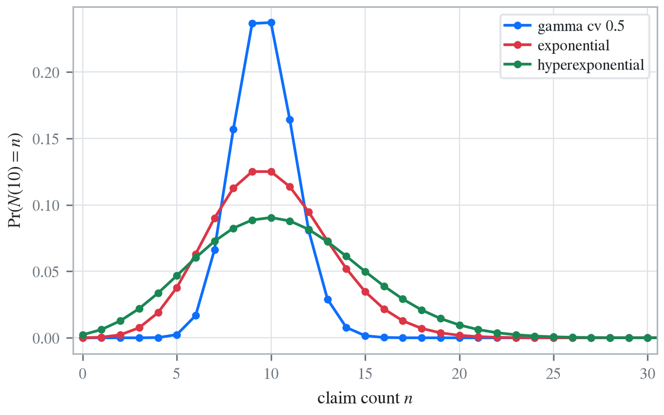

Renewal count moments and their asymptotic expansions

The table compares the computed mean and variance of the renewal count over ten years with the asymptotic expansions, for gamma, exponential, and hyperexponential waits with mean one. The wait moments are taken from the wait law stored in the frequency: wait_components lists its Severity objects and wait_weights their mixture weights. At \(T=10\) the asymptotic mean and variance match the computed moments to five figures or better.

def asymptotics(b):
    f = b.frequency
    w = np.atleast_1d(f.wait_weights)
    m1, m2, m3 = w @ np.array([sev.moms() for sev, *_ in f.wait_components])
    s2, c3, T = m2 - m1 ** 2, m3 - 3 * m1 * m2 + 2 * m1 ** 3, f.years
    return {'wait cv': s2 ** 0.5 / m1, 'mean': b.est_m,
            'asymptotic mean': T / m1 + (s2 - m1 ** 2) / (2 * m1 ** 2),
            'variance': b.est_var,
            'asymptotic variance': s2 * T / m1 ** 3 + 1 / 12
            + 5 * s2 ** 2 / (4 * m1 ** 4) - 2 * c3 / (3 * m1 ** 3)}

df = pd.DataFrame({k: asymptotics(b) for k, b in books.items()}).T
GT(df.rename_axis('wait law'), float_format='.6f')

wait law	wait cv	mean	asymptotic mean	variance	asymptotic variance
gamma cv 0.5	0.500000	9.625000	9.625000	2.578125	2.578125
exponential	1.000000	10.000000	10.000000	10.000000	10.000000
hyperexponential	1.414214	10.499977	10.500000	18.750296	18.750000

Discrete waits

The dwait clause takes outcomes and probabilities, like dsev. Unit waits over three years give exactly three claims, since the arrival on the horizon counts, and the count has CV zero. A zero wait is a simultaneous claim, so dwait [0 1] [0.5 0.5] produces clusters of claims, and over two years the mean count is 5. Probabilities summing to \(0.9\) with ! leave a defect of \(0.1\): each wait is infinite with probability \(0.1\), and no claim arrives after the first such wait.

for program in ['agg Det 3 years dsev [1] dwait [1]',
                'agg Clu 2 years dsev [1] dwait [0 1] [0.5 0.5]',
                'agg Ter 2 years dsev [1] dwait [1 2] [0.4 0.5] !']:
    b = build(program)
    print(f'{program:48s} mean {b.est_m:6.4f}  cv {b.est_cv:6.4f}  '
          f'defect {b.frequency.wait_defect:.1f}')

agg Det 3 years dsev [1] dwait [1]               mean 3.0000  cv 0.0000  defect 0.0
agg Clu 2 years dsev [1] dwait [0 1] [0.5 0.5]   mean 5.0000  cv 0.4899  defect 0.0
agg Ter 2 years dsev [1] dwait [1 2] [0.4 0.5] ! mean 1.0600  cv 0.4777  defect 0.1

An aggregate with a renewal count

A renewal count combines with any severity \(X\), as a Poisson count does. The aggregate variance is \(\mathsf{P}N\,\mathrm{Var}X + \mathrm{Var}N\,(\mathsf{P}X)^2\), so regular arrivals narrow the aggregate. The example has gamma waits with mean \(1/2\) and CV \(1/2\) over five years, an expected 9.625 claims, compared with a Poisson count with the same mean on the same grid, and at 300 rate sets a premium of 1,500. The renewal count has CV 0.17 against 0.32 for the Poisson, and the aggregate CV is 0.36 against 0.46.

r = build('agg Ren 5 years at 300 rate sev lognorm 100 cv 1 wait gamma 0.5 cv 0.5')
p = build(f'agg Po {r.n:.4f} claims sev lognorm 100 cv 1 poisson', bs=r.bs, log2=r.log2)
qd(r)
qd(p)
print(r.pprogram)
print(f'premium {r.exp_premium:,.0f}')

Aggregate object: Ren. Frequency distribution renewal. Severity lognorm,
[0, inf), subexponential right tail. Updated with bucket size 1/4 and
log2 = 16. Validation: not unreasonable.

      Mean     SD      CV    Skew    P01 Median   P99
X                                                    
Freq 9.625 1.6057 0.16682 0.15098                    
Sev    100    100       1  3.9998  10.25  70.75 490.5
Agg  962.5 349.33 0.36294  1.0992 373.75 911.25  2029
Aggregate object: Po. Frequency distribution poisson. Severity lognorm,
[0, inf), subexponential right tail. Updated with bucket size 1/4 and
log2 = 16. Validation: not unreasonable.

      Mean     SD      CV    Skew   P01 Median    P99
X                                                    
Freq 9.625 3.1024 0.32233 0.32233                    
Sev    100    100       1  3.9998 10.25  70.75  490.5
Agg  962.5 438.75 0.45584 0.91166   208 903.25 2256.5
agg Ren
  5 years at 300 rate
  sev lognorm 100 cv 1
  wait gamma 0.5 cv 0.5
premium 1,500

The renewal aggregate has the slightly higher median, 911 against 903. Its upper quantiles are lower, and at the 99.9% level it is 2,701 against 2,967 for the Poisson.

ps = [0.5, 0.9, 0.99, 0.999]
df = pd.DataFrame({'renewal': [r.q(x) for x in ps], 'poisson': [p.q(x) for x in ps]},
                  index=pd.Index([f'{x:g}' for x in ps], name='p'))
GT(df, float_format=',.1f')

p	renewal	poisson
0.5	911.2	903.2
0.9	1,415.2	1,540.5
0.99	2,029.0	2,256.5
0.999	2,700.8	2,967.0

Refused programs

The years exposure and the wait or dwait clause are paired by the grammar, so either one without the other is a parse error. The horizon must be a single number, not a vector.

refuse('agg X 10 years dsev [1] poisson',
       'agg X 10 claims dsev [1] wait expon',
       'agg X [5 10] years dsev [1] wait expon')

DecL parse error at line 1, column 27: Unexpected 'poisson'.
DecL parse error at line 1, column 28: Unexpected 'wait'.
DecL: years in a years (renewal) exposure must be a scalar, not a vector

Footnotes

1. From aggregate 1.0